the Creative Commons Attribution 4.0 License.
the Creative Commons Attribution 4.0 License.
 | 09 Nov 2021
Co-varying effects of vegetation structure and terrain attributes are responsible for soil respiration spatial patterns in a sandy forest–steppe transition zone
Szilvia Fóti
László Körmöczi
Dóra Petrás
Levente Kardos
János Balogh
Forest–steppe habitats in central Hungary have contrasting canopy structure with strong influence on the spatiotemporal variability of ecosystem functions. Canopy differences also co-vary with terrain feature effects, hampering the detection of key drivers of carbon cycling in this threatened habitat. We carried out seasonal measurements of ecosystem functions (soil respiration and leaf area index), microclimate and soil variables as well as terrain features along transects for 3 years in poplar groves and the surrounding grasslands. We found that the terrain features and the canopy differences co-varyingly affected the abiotic and biotic factors of this habitat. Topography had an effect on the spatial distribution of soil organic carbon content. Canopy structure had a strong modifying effect through allocation patterns and microclimatic conditions, both affecting soil respiration rates. Due to the vegetation structure difference between the groves and grasslands, spatial functional diversity was observed. We found notably different conditions under the groves with high soil respiration, soil water content and leaf area index; in contrast, on the grasslands (especially in E–SE–S directions from the trees) soil temperature and vapor pressure deficit showed high values. Processes of aridification due to climate change threaten these habitats and may cause reduction in the amount and extent of forest patches and decrease in landscape diversity. Owing to habitat loss, reduction in carbon stock may occur, which in turn has a significant impact on the local and global carbon cycles.
- Article
(2953 KB) - Full-text XML
- BibTeX
- EndNote


Due to global climate change, extreme weather events (i.e., heat waves and extreme rainfalls) frequently occur worldwide. They are expected to have a major impact on the structure of forest ecosystems and on the dynamics of environmental factors and functional variables in forest patches and nearby open areas (Chatterjee and Jenerette, 2011; Cunningham et al., 2006; Shi et al., 2011). Transition zones (e.g., edges, forest patches with grasslands) with distinct vegetation physiognomy and plant species compositions could be sensitive habitats (Erdős et al., 2014), as adjacent communities may respond differently to extreme events, depending on their sensitivity and stability. Despite this sensitivity, the ecosystem functions (e.g., soil respiration) of these transition zones are less studied among temperate ecosystems (Erdős et al., 2018).
Soil respiration (Rs) can be considered to be one of the most important functional variables of ecosystems, consisting of respiration by various organisms and showing the overall biological activity of the soil (Jassal and Black, 2006; Shi et al., 2011). The two main components of Rs are autotrophic respiration (Raut) by plant roots and root-associated microbes and heterotrophic respiration (Rhet) by microbes and animals in the soil (Balogh et al., 2016).
Soil factors generally influence the temporal and spatial variance of Rs rate, e.g., soil organic carbon content (SOC), soil physical and chemical properties (texture, bulk density, pH, etc.). The density and activity of plant roots through Raut as well as the activity of soil microbial biomass through Rhet have great influence on Rs rate too (Lellei-Kovács et al., 2016; Michelsen et al., 2004; Mitra et al., 2019; Thomas et al., 2018). The share of Rs components is largely dependent on these variables (Hu et al., 2001; Moyes and Bowling, 2016; Raich and Tufekcioglu, 2000; Tang et al., 2020), responding to the changes of environmental factors differently (Balogh et al., 2016; Shi et al., 2011). Among the soil parameters, Rs shows a positive temporal relationship with soil temperature (Ts) and soil water content (SWC) (Balogh et al., 2015; Lellei-Kovács et al., 2016; Moyes and Bowling, 2016; Shi et al., 2011; Tang et al., 2020). Thus, seasonal changes in soil parameters play a significant role in defining seasonal differences in soil CO2 emission (Hao et al., 2010; Herbst et al., 2009; Mitra et al., 2019; Raich and Tufekcioglu, 2000; Thomas et al., 2018).
SWC and Ts strongly influence the growth and distribution of plant species as well (Cuena-Lombraña et al., 2018; Latif and Blackburn, 2010; Potter, 2014). In addition, the vegetation composition and structure are crucial determinant factors of Rs rate by influencing canopy microenvironment (Chatterjee and Jenerette, 2011; Petrone et al., 2008), soil microclimate and soil organic matter through plant residue input (Stoyan et al., 2000). Consequently, transitions in the vegetation types cause sharp changes in the spatial and temporal variability of the canopy's carbon assimilation, governing allocation patterns and litter production, thus resulting in different levels of stored terrestrial carbon belowground (Chen et al., 2011). Several previous studies (Huang et al., 2020; Michelsen et al., 2004; Shi et al., 2011; Thomas et al., 2018) showed Rs dissimilarities between different vegetation types (e.g., woody vegetation vs. grassland). Grasses allocate greater amounts of carbon for growth and typically produce a larger amount of readily decomposable litter, while trees generally allocate more carbon to structural tissues and produce smaller amounts of longer-lasting, nutrient-poor litter (Moyes and Bowling, 2016; Raich and Tufekcioglu, 2000). Related to relative carbon allocation, Rs rates were usually found to be lower in grasslands than in forests (Moyes and Bowling, 2016; Thomas et al., 2018). Woody vegetation has the largest carbon stocks among vegetation types; thus the transition of woody vegetation to grasslands via natural (i.e., forest–steppe mosaics) or unnatural (deforestation) mechanisms is of great importance. This type of land cover change was considered to be one of the most important drivers of global Rs changes (Huang et al., 2020).
Forest–steppe habitats in central Hungary are naturally fragmented transition zones, where a mosaic of forests with grasslands can develop, as neither of them has a decisive advantage over the other (Erdős et al., 2018). This type of ecosystem has a very sharply separated structure between the forest patches/groups of trees and the open grasslands, which are in close contact with each other through biotic and abiotic factors (Süle et al., 2020). The strong abiotic (i.e., soil water content, SWC) differences in the edges prevent the forest's expansion and development by constraining its growth (Erdős et al., 2014). The sandy forest–steppe vegetation type is in danger of total disappearance in the near future due to the aridification of this region (Pongrácz et al., 2014). Hence, improving our knowledge about ecosystem functioning in this habitat could provide new insights into the effects of global change and a key to preserving these habitats and maintaining landscape diversity (Erdős et al., 2014, 2020; Morecroft et al., 1998).
The vegetation patterns in open landscapes such as sandy grasslands are often influenced by elevation and environmental factors determined by micro-topography. Surface altitudinal heterogeneity not only is a key factor in determining not only the spatial patterns of SWC and Ts but also has a strong connection with the microclimate above the soil surface. Actually, the abiotic factors of the landscape/habitat related to terrain attributes (e.g., slope, altitudinal differences, aspect) and the subsequent distribution of plant species (Cuena-Lombraña et al., 2018; Hohnwald et al., 2020; Latif and Blackburn, 2010; Potter, 2014) mutually influence each other (Alexander et al., 2016). The slopes and altitudinal differences can be closely related to water accumulation and surface runoff, which were found to influence functional spatiotemporal patterns of the vegetation (Fóti et al., 2020; Lassueur et al., 2006). Slopes with different orientation are exposed to different physical effects (e.g., predominant wind direction and irradiation). The main difference between north- and south-facing slopes resides in their shade duration, due to the different amounts of incoming solar radiation (Alexander et al., 2016; Fóti et al., 2020), and the west side of a grove could be colder than the east side during a diurnal period (Süle et al., 2020). This variability in shading causes significant variation in plant composition (Erdős et al., 2014), with the subsequent differences in microclimate giving evidence of a mutual spatiotemporal effect. Although the abovementioned publications show evidence of terrain attributes' effects, little is known about how a tree group acts on their covariation with shading effects.
The most important microclimatic components usually examined with Rs variability include air temperature and air humidity (Matlack, 1993; Potter, 2014) and vapor pressure deficit (VPD) (Bolton, 1980; Chen et al., 1995; Süle et al., 2020). VPD can be an important limiting factor in plant growth because above a certain threshold photosynthetic CO2 uptake is strongly limited due to stomatal closure to prevent water loss (Novick et al., 2016; Shamshiri et al., 2018; Young and Mitchell, 1994). In our previous study (Süle et al., 2020) we found that at a 3 kPa threshold value of VPD species composition differences between the grove and the adjacent grassland areas were accompanied by differences in their VPD distribution (Süle et al., 2020).
The objectives of this study were (1) to examine the spatial variability of the functional responses of a grove with the surrounding grassland in terms of Rs and canopy characteristics in different phenological stages as well as (2) to link these responses to the background factors given by the spatially co-varying effects of the habitat's terrain features and the grove. Our main question was as follows: which are the main influencing factors of soil respiration in an ecosystem with such a large vegetation structure heterogeneity?
2.1 Study area
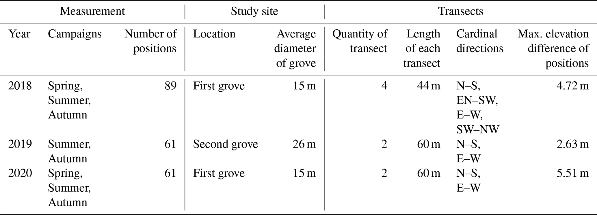
Our study sites were situated in central Hungary (Fülöpháza region of the Kiskunság National Park). The 10-year (2010–2020) temperature and precipitation averages of this region were 11.5 ∘C and 622.17 mm, respectively (National Meteorological Service, Fülöpháza Meteorological Station). Humus-poor sandy soils are characteristic in this region, which have extremely low water-holding capacity and soil organic matter content (Erdős et al., 2014). Due to these poor soil features, precipitation drains quickly, so the amount of water in the soil available for plants is very small. Two groves of poplar (Populus alba) and their surrounding grasslands were selected for this study (Fig. 1) to represent the sharp vegetation structure differences of the forest–steppe habitat. Relief maps as well as sampling positions of the first grove ( N, E, 107 m a.s.l) and second grove ( N, E, 106 m a.s.l.) can be seen in Fig. 2. Measurements of environmental and functional variables were performed in intersecting transects with different cardinal directions, forming together a star and cross-shape sampling arrangement with the group of trees in the middle (Fig. 2, Table 1).
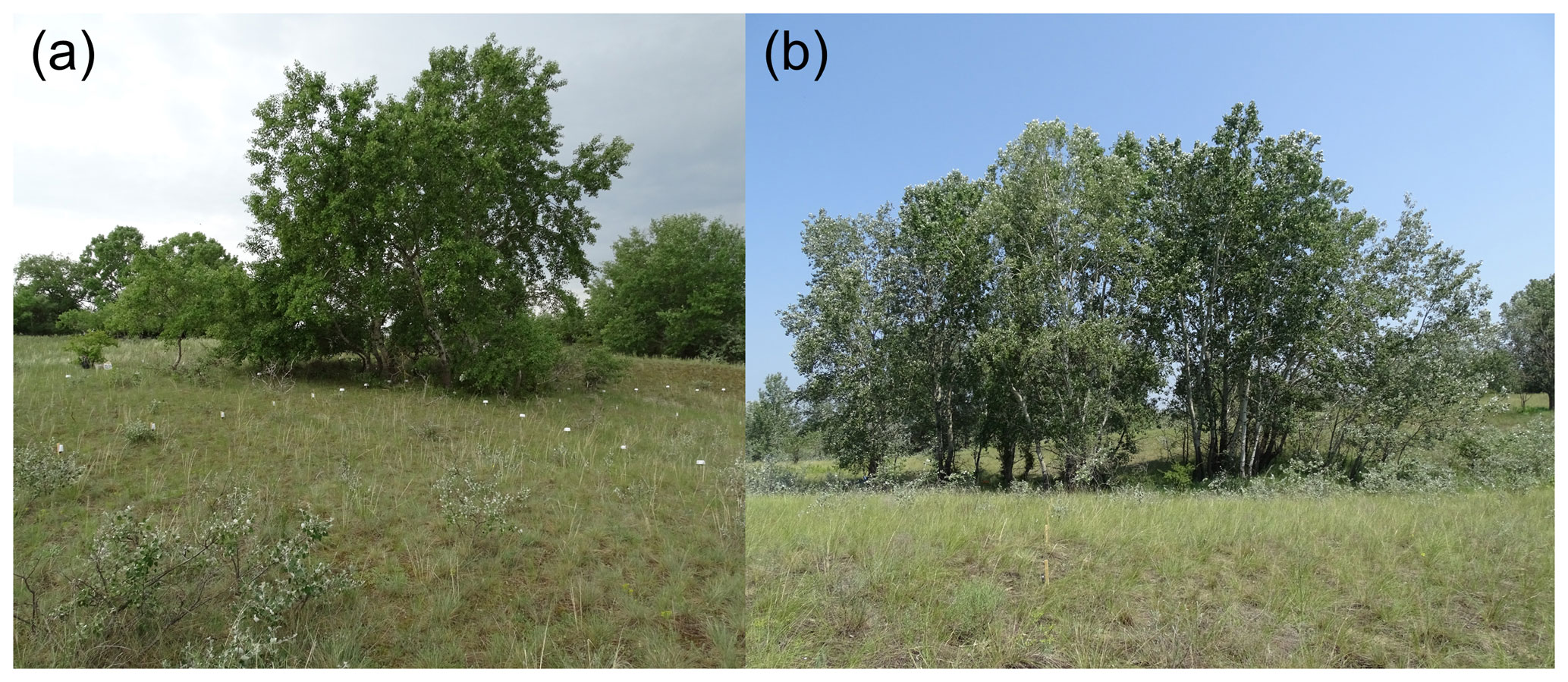
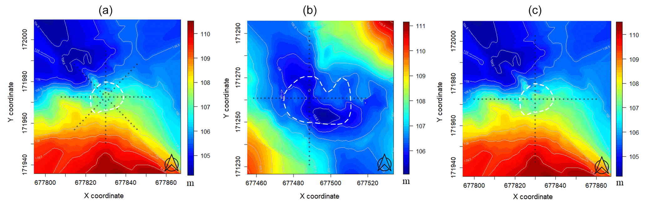
Figure 2Digital elevation models and sampling arrangements of the sites (a: first grove in 2018; b: second grove in 2019; c: first grove in 2020; white dashed line: visual tree edges; black dots: sampling positions). Coordinates refer to the Hungarian Unified National Projection system and are given in meters.
2.2 Measurements of soil parameters and functional variables
Measurements of soil parameters and functional variables were performed along transects with 2 m intervals between the measurement positions. Rs and Ts were measured by an EGM-4 infrared gas analyzer (PP Systems, UK). SWC was measured by a FieldScout TDR 300 (FieldScout, USA) with a 3.0 in. (7.62 cm) rod. Leaf area index (LAI) was measured by an ACCUPAR LP-80 ceptometer (METER Group, USA). Manual measurements were taken near noon and lasted about 1.5 h (Fóti et al., 2018). All of the statistical evaluation was performed in R (R Core Team, 2018). We used standardization (Hmisc package: Harrell and Dupont, 2020) on the variables mentioned above for principal component analysis (PCA biplot; vegan package: Oksanen et al., 2019).
To separate Rhet and Raut components, we calculated the mean Rs from the whole dataset of each measuring campaign. From the LAI–Rs linear regression, we determined the y-axis intercept (where LAI is theoretically 0) for each measurement campaign, considering it as the average Rhet rate. Therefore, we calculated Raut rate as the difference between mean Rs rate and the Rhet rate.
In each measurement year, bulk soil samples were taken from the upper 10 cm at the measurement positions along the transects. SOC (%) of sieved soil was determined by sulfochromic oxidation and loss on ignition (Ivezić et al., 2016).
2.3 Microclimate measurements and vapor pressure deficit
Air temperature and air humidity were measured in the herb layer with a sensor network along the transects at 2 m intervals for 48 h (1 min resolution) during each measurement campaign. The data loggers were placed 20 cm above the soil surface, at the average height of the herbaceous vegetation. Crossbow MICA XM2110CA mote (Crossbow Technology Inc., Milpitas, CA, USA), UNI-T UT330B Mini USB temperature humidity logger (UNI-TREND Technology CO Ltd., Guangdong, China) and Voltcraft DL-120TH USB temperature humidity logger (Voltcraft, Hirschau, Bavaria, Germany) were used. The sensors were shielded with a white plastic plate to avoid direct solar radiation. The sensors were calibrated before the measurements. We selected precipitation-free measurement periods, but it rained during the measurements in October 2020. The main changes in the weather conditions were described by observation (e.g., clouds' shading and movement) and recorded manually. The location of the visual edges of the grove, the positions of bushes and trees in the surrounding area, and the shadow of the groves were described by observation and were also recorded manually.
VPD was computed (Hmisc package: Harrell and Dupont, 2020) from the relative air humidity (RH) and air temperature (t) according to the formula developed by Bolton (1980):
with t in degrees Celsius, RH in percent, and VPD in pascals.
We used the average of per minute VPD in the 11:00–13:00 LT period for this study to examine the same period covered by the other measurements during the day. We also used standardization (Hmisc package: Harrell and Dupont, 2020) on VPD for principal component analysis (PCA biplot; vegan package: Oksanen et al., 2019).
2.4 Measurement with GPS, digital elevation model (DEM) processing and terrain attribute calculations
Coordinates and altitude of measuring positions along the transects were recorded by high-precision STONEX S8 PLUS GPS (STONEX Srl., Paderno Dugnano, Italy).
We used spline interpolation (akima: Akima et al., 2016, and field packages: Nychka et al., 2017) of the measured altitude data to generate DEMs of 0.4 m resolution for the groves, which could serve as input raster data for terrain attribute calculations. Although DEMs in general are built on the basis of data collected by remote sensing techniques, they may equally be built from land surveying by GPS receivers. These interpolation maps can be seen in Fig. 2 together with the measuring positions. The maps lie on 183 (first grove) and 106 (second grove) randomly measured data, respectively.
Four terrain attributes were calculated for the best characterization of the surface with the least potential co-variance between the selected attributes and the ones which were found to be applicable for a range of terrain complexities. For a more detailed description of the calculations please refer to Fóti et al. (2020). We used RSAGA (Brenning et al., 2018) and raster packages (Hijmans, 2018) for the terrain attribute analyses mentioned below. We calculated Spearman correlation coefficients (Hmisc package: Harrell and Dupont, 2020) between PCA scores of the biplots mentioned earlier, SOC and these terrain attributes.
Standard deviation of elevation (SD) was calculated by “mixed scaling” (see Behrens et al., 2018) for a smoothed DEM of 1.5 m (to approximately meet the sampling resolution) by 5×5 box blur kernels as the neighborhood as follows:
where zi values are the elevations of the correspondent R radius while is the mean elevation within R. SD describes the heterogeneity and local surface roughness within the raster.
For slope- and aspect-derived easterness and northness, we used eight neighbors, as suggested by Lecours et al. (2017):
Slope (Sl) expresses the rate of change in elevation between positions; it is the tangent (vertical “rise” divided by horizontal “run”) of a surface angle to the horizontal in degrees.
Easterness and northness (east, north) aspect is the compass direction that a slope faces, derived from the maximum downslope rate of change in a value from a raster cell to its neighbors. It is a circular variable ranging clockwise from 0 to 360∘ from the north (both 0 and 360∘ meaning N-facing slope, 90∘ meaning E-facing slope; Ritter, 1987). In ecology, use of sine (easterness) and cosine (northness) of aspect is more frequent because they provide a continuous gradient of east–west and north–south directions, respectively. Northness and easterness with the values close to +1 mean that the slope is northward and eastward in general, while values close to −1 mean a generally south- and west-facing slope.
3.1 Measuring circumstances (National Meteorological Service, Fülöpháza meteorological station)
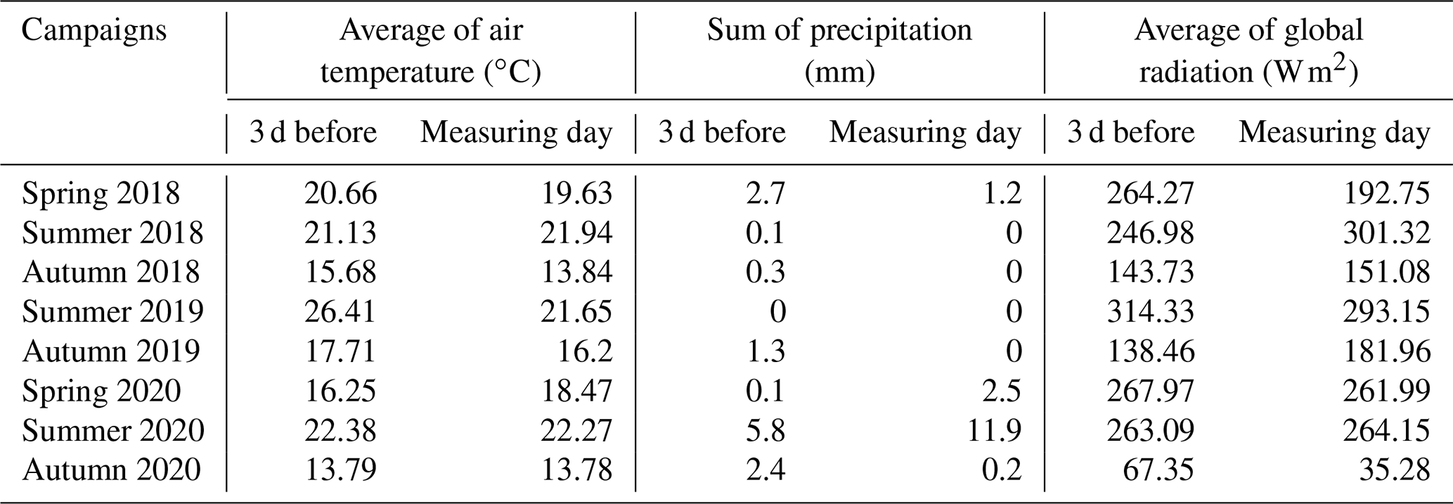
Daily average temperatures and daily precipitation sums are presented in Fig. 3 for the study period between May 2018 and October 2020. The first measuring campaign was usually scheduled for spring, the second was in mid-summer and the third was in autumn. We present the summary of the preceding meteorological conditions of the measurement campaigns in Table 2. During spring 2018 and all of the 2020 measurement campaigns it had rained before the measuring day. The amount of daily precipitation observed on the day of the measurement in summer 2020 fell during the previous night, but no precipitation occurred during the measurements. During the autumn 2020 measurement campaign, the global radiation was very low compared to the other measurement periods.
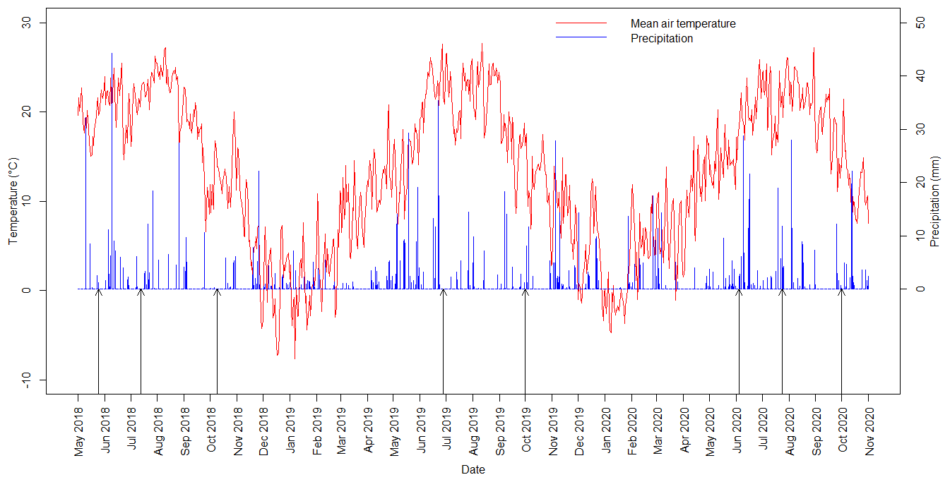
Figure 3Daily averages of air temperature and daily sums of precipitation during the study period with the measuring days (black arrows), spring 2018–autumn 2020, at the Fülöpháza site.
Table 2Averages of air temperature, sums of precipitation and averages of global radiation at the measuring campaigns and 3 d before them.
3.2 Relationships between the measured variables
Rs showed significant positive correlation with SWC (P<0.001, R2=0.13) (Fig. 4a) and LAI (P<0.001, R2=0.28) (Fig. 4c) and showed negative correlation (P=0.059, R2=0.004) with Ts (Fig. 4b). The highest Rs values were observed in summer 2019 (23.99 ). In general, Rs was the lowest (0.13 ) in the autumn phenological stages at relatively low temperatures (13.2 ∘C) and low LAI (0.15 m2 m2). No significant relationship was found between Ts and Rs (Fig. 4b) due to the high temperatures measured in summer 2018 coupled with low water availability. LAI showed significant negative correlation (P<0.001, R2=0.08) with VPD (Fig. 4d). No separated data group could be found in these regressions (Fig. 4), except autumn 2020, which was completely separated from the other phenological stages in Fig. 4d. However, characteristic groupings can be seen by phenological stages in Fig. 4b, pointing to the differences in the environmental conditions during measuring campaigns. The points of Fig. 4b and d have a hyperbolic shape.
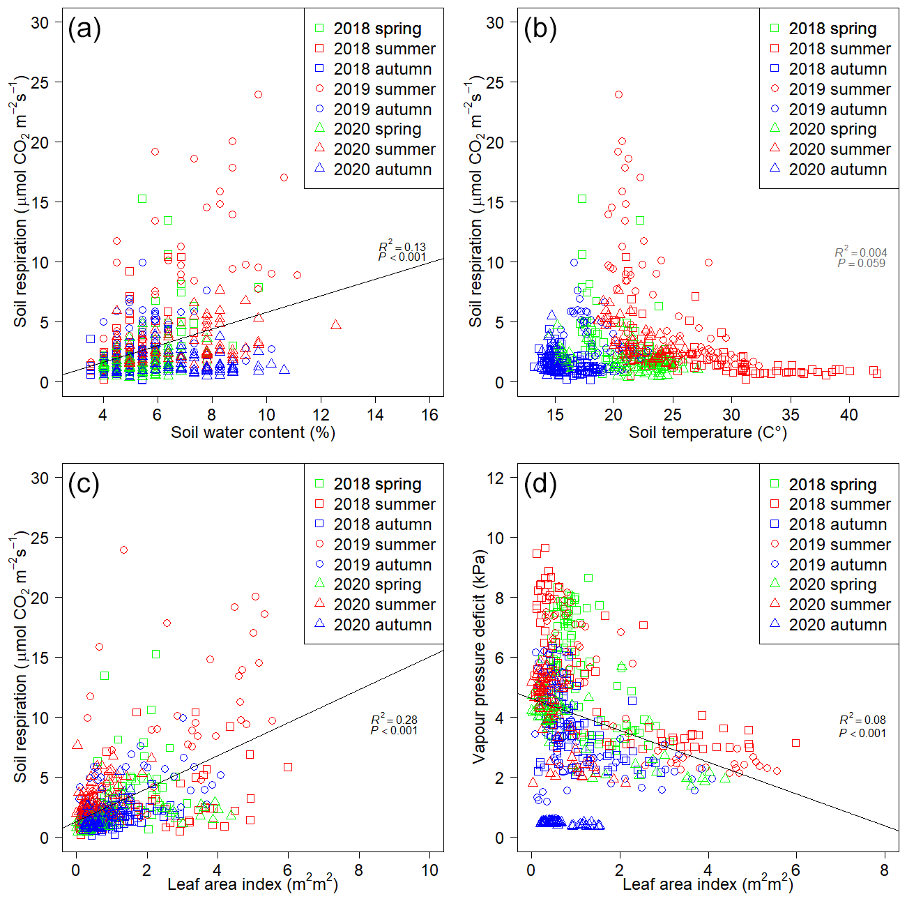
Figure 4Relationships between variable pairs of the measurement campaigns. Pairs: soil respiration vs. soil water content (a), soil respiration vs. soil temperature (b), soil respiration vs. leaf area index (c) and leaf area index vs. vapor pressure deficit (d).
3.3 Rs component rates
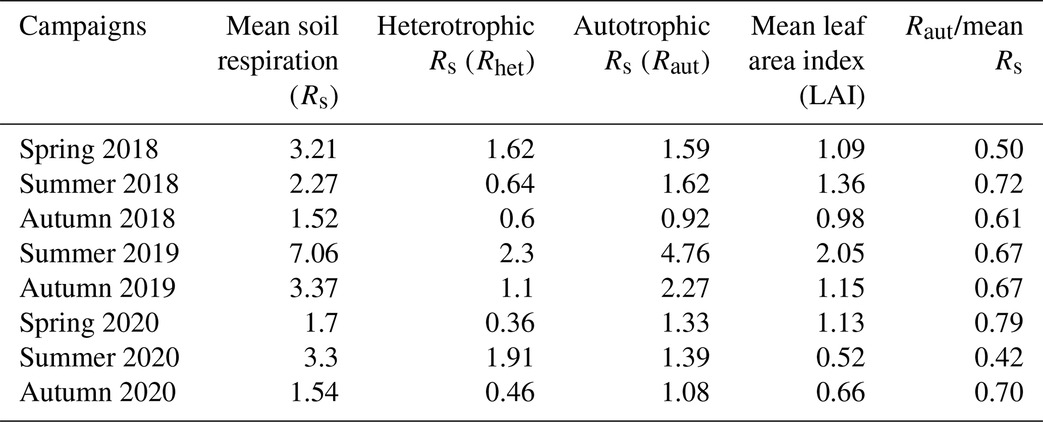
A characteristic trend can be observed in the Rs component rates of the measurement campaigns (Table 3). Within a year, spring and summer phenological stages were similar to each other, with a slightly higher autotrophic respiration component in summer, while this component was the lowest in autumn. The year 2019 had higher values than the other two surveyed periods. Raut seemed to closely follow LAI.
Table 3Rates of soil respiration and its components with leaf area-index during the measurement campaigns.
3.4 Connections between the variables and vegetation physiognomy
PCA biplots (Fig. 5) were used to analyze relationships among variables. Based on this analysis, in every measurement campaign the positions below the groves were notably separated from the positions in the surrounding grasslands, especially the positions lying eastward and southward from the trees. However, in the autumn phenological stage, the positions of the two vegetation types became less separated, especially in the first 2 years, when grassland positions north of the trees overlapped remarkably in PCA space with below-canopy positions. Among the studied variables, Rs showed a positive relationship with SWC and LAI, while it showed a negative relationship with Ts and VPD, as shown by PCA loadings along the first axis. The second axis separated SWC, Rs and LAI in any potential combination, reflecting the same underlying causes with some variation in the actual signs of the loading, although the most frequent case was in which SWC and Rs were separate from LAI. Mainly, the loadings of Rs–SWC–LAI correlated positively with the distribution of the new PCA scores originating from the positions of the groves, while the distribution of the grasslands' positions followed Ts–VPD loadings, especially those that can be considered warmer, including the E, SE and S directions from the trees, except for at the 2020 autumn phenological stage due to loading of SWC.
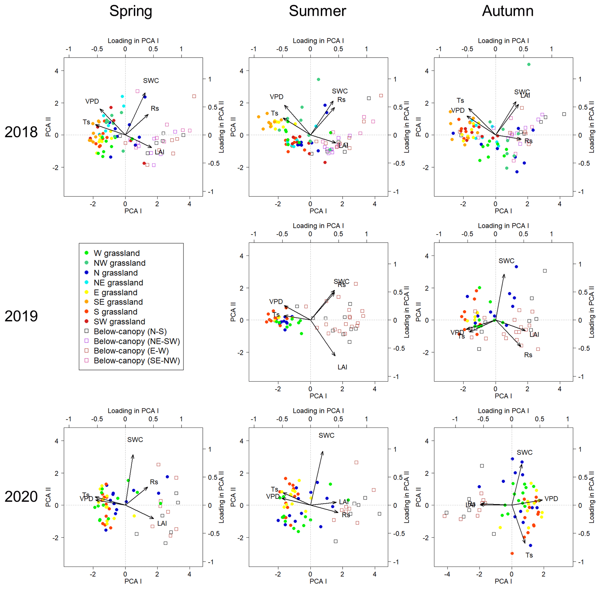
Figure 5PCA biplots of the measurement campaigns with separation of the measuring positions below (open square symbols) and surrounding (closed spots with cold–warm colors according to the cardinal directions) the groves. Variables: soil respiration (Rs), soil water content (SWC), leaf area index (LAI), soil temperature (Ts) and vapor pressure deficit (VPD). Cardinal directions: west (W), northwest (NW), north (N), northeast (NE), east (E), southeast (SE), south (S) and southwest (SW).
3.5 Correlations between the variables, soil organic carbon and terrain attributes
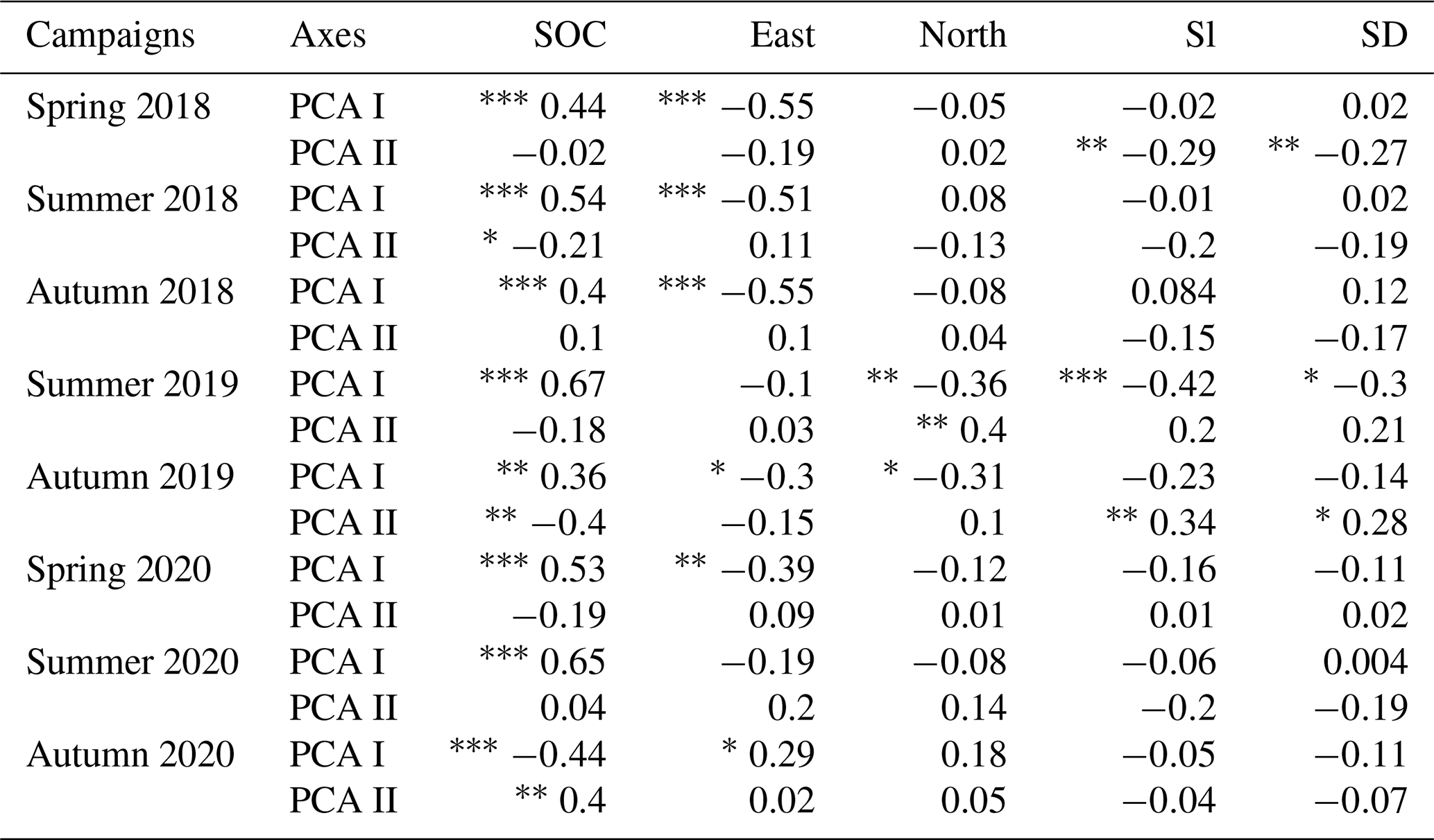
Soil organic carbon content showed strong positive correlation with the PCA I axes of Fig. 5 of every measurement campaign, except in autumn 2020, where it showed strong negative correlation with the PCA I axis and positive significant correlation with the PCA II axis (Table 4). This difference was in good agreement with the orientation change of the loadings in Fig. 5 (autumn 2020 biplot). In the campaigns of 2018 and 2020 eastern orientation had a significant negative correlation with PCA I axes (and the opposite again in the case of autumn 2020), similarly to the findings in the biplot analysis, with “warmer” grassland positions matching Ts–VPD loadings the most. In addition, Sl and SD showed negative correlations with PCA II axes in the 2018 spring phenological stage, which means that larger Rs and SWC were measured at smaller elevation differences with slight slopes, although this effect was not detectable in the measuring campaign of 2020. This was probably due to the rainy days before the measuring occasion (see Table 2), masking the effects of the surface. At the study site in 2019, north showed a negative correlation with PCA I axes on both occasions, while Sl and SD showed a negative correlation with PCA I axes in spring and a positive correlation with PCA II axes in autumn. These correlations again suggest larger Ts–VPD values at south-facing directions and also larger Rs and LAI values in those positions with less surface heterogeneity.
Table 4Spearman correlation coefficients between PCA scores of Fig. 4, soil organic carbon (SOC) and terrain attributes (: P<0.001, : P<0.01, ∗: P<0.05).
The vegetation composition and horizontal and vertical structures of ecosystems are crucial determinant factors of the environmental and functional variables influencing, among others, the air and soil microclimate and soil chemical parameters (Huang et al., 2020; Mitra et al., 2019; Thomas et al., 2018). The structural differences in the vegetation types cause spatiotemporal variability in the assimilation and allocation patterns, with subsequent effects on the soil carbon stocks.
4.1 The spatiotemporal explanatory factors of Rs
The responses of Rs to soil moisture and Ts were investigated in several studies, which already reported that the correlation between Rs and Ts as well as SWC and Ts differed in temporal and spatial studies (Allaire et al., 2012; Almagro et al., 2009; Fóti et al., 2020; Herbst et al., 2009; Lellei-Kovács et al., 2016; Moyes and Bowling, 2016; Shi et al., 2011; Tang et al., 2020). Our study is consistent with these findings, because Rs showed positive correlation with SWC and LAI. Although it was often found that there is a positive correlation between Rs and Ts in temporal datasets (Balogh et al., 2019; Savage et al., 2013), based on our entire dataset with sharp vegetation structural differences (Fig. 4b), we could not detect this kind of relationship. However Rs showed negative correlation with Ts and VPD in space by measuring campaigns (Fig. 5) similarly to the findings of other spatial studies (Fóti et al., 2014; Herbst et al., 2009). VPD showed negative correlation with LAI both in time and in space and very often had the opposite loading of SWC, Rs and LAI in the PCA analysis of spatial data. The below-canopy area had higher Rs and LAI with lower air temperature and Ts due to the microclimate below the complex vegetation structure and higher biomass with trees and bushes. In contrast, the grassland had higher Ts and VPD with lower Rs due to the higher irradiation (Huang et al., 2020; Moyes and Bowling, 2016; Thomas et al., 2018).
4.2 The components of Rs
We found seasonal differences in Rs and component rates within a year. In sandy forest–steppe habitat, which is an ecosystem with a semiarid climate and predominantly open vegetation with low biomass (Erdős et al., 2020), the autumn phenological stage may already be a dormant period. It contrasts with other dry sandy grasslands (Balogh et al., 2016) and mesic meadows with trees (Moyes and Bowling, 2016), which have higher biomass and higher organic carbon content. In a closed dry sandy grassland (Balogh et al., 2016) there could be an active re-greening period with higher Rs rates in autumn than in the summer. Besides, the correlation between Raut and the seasonal variation in LAI reflected the effect of vegetation structure on the ecosystem functioning and revealed the strong modifying effect of plant CO2 uptake on soil respiration.
4.3 The influence of cardinal directions and topography
Several studies referred to north–south as the coolest–warmest temperature gradient (Erdős et al., 2014; Hohnwald et al., 2020; Latif and Blackburn, 2010; Matlack, 1993) and also highlighted that northern areas of edges and the surrounding open areas showed similarities in microclimate and vegetation composition with the forest interior (Erdős et al., 2014). In our study, the reason for the grouping of grassland positions is the difference in Ts and VPD values, which can be traced back to the temperature gradient. This also caused the scatter of positions of the grassland side north of the trees near the grove.
In addition, the warmer areas matched with the easterness terrain attribute, and the Ts–VPD variables aligned with the south-facing slope terrain attribute. Also, the spatial distribution of SOC followed the spatial change of vegetation structure because the grove had higher carbon content. Our results were in good agreement with the findings that woody vegetation has the largest carbon stock among the vegetation types (Huang et al., 2020; Moyes and Bowling, 2016; Tang et al., 2020); thus the transition of woody vegetation to some short vegetation type, for example in forest–steppe mosaics, is of great importance. On the other hand, surface heterogeneity was lower under the grove due to the fact that the seeds of tree species in this habitat can only germinate in ideal depressions, where a sufficient amount of water can accumulate (Erdős et al., 2014). In the context of spatial heterogeneity, deeper positions contain more carbon due to accumulation, resulting in higher Rs activity and SWC (Fóti et al., 2020). These parameters indicated the functional differences within the study sites, mostly between the grove and the surrounding grasslands but also between the grassland areas based on their cardinal directions.
4.4 The effect of the heterogeneous vegetation
We found that the groves were separated from the surrounding grasslands based on the measured variables, except in the autumn phenological stage due to the lower irradiation. In this phenological stage, the grassland heated up less, Ts was lower and soil moisture evaporated at a lower rate. The shade of the group of trees also lasted longer on the grassland in autumn, yet a less marked difference could be observed between the grassland and the grove. This is in good agreement with the results of the study conducted by Thomas et al. (2018), where solar radiation, air and soil microclimate parameters showed the same trend during the phenological stages of a year due to the shade of the trees. A similar seasonal trend was also observed by Moyes and Bowling (2016) in the case of Ts and SWC. Opposite orientations of Rs–SWC–LAI and Ts–VPD loadings along PCA I axes in the 2020 autumn phenological stage can probably be attributed to the low global radiation on the measuring day.
4.5 The main influencing factors of Rs in forest–steppe habitat
Topography sometimes had a very clear modifying effect on abiotic and biotic factors of ecosystems in connection with cardinal directions, exposure, spatial heterogeneity and carbon spatial distribution (Alexander et al., 2016; Fóti et al., 2020; Lassueur et al., 2006). Based on our results, the co-varying effects of the habitat's terrain features and of the grove could be observed. We detected mixed effects of the topography and the shading of the grove on the measured variables; thus topographical effects can be masked by conditions related to the physiognomy of the forest–steppe. We highlight that the extent of the effect of topography may also differ for groves with slightly different locations and vegetation structure, as well as for slightly different sampling resolution and arrangement (Körmöczi et al., 2016). In addition, the distribution of the “warmer” and “colder” grassland positions in the PCA biplots in the context of the environmental and functional variables was a great indicator of the shadowing effect of the grove, which, in addition to the topography, also had a strong effect on these factors (Erdős et al., 2014, 2017; Süle et al., 2020). Topography and shading caused variability in the functional responses of the ecosystem. Overall, the variation in the functional responses was quite small, and the temporal trends were the same, although rainy weather and temporal variability had a strong influencing power.
This study provided information on the ecosystem functioning of a small group of trees with the surrounding grassland as a transition zone in a forest–steppe habitat. We described the functional responses and the influential effects of topography and shading.
The terrain features of the habitat and the physiognomy of the grove had a co-varying influence on the abiotic and biotic factors of this habitat. Topography had a clear effect on the ecosystem functioning and carbon spatial distribution, but we also highlighted the importance of locations, vegetation structure, weather and seasonal differences. The responses generally had similar characteristics and temporal trends, such as the vegetation structure showing a strong correlation with Rs and the components of Rs along the investigated seasons. The vegetation structure also influenced the microclimate, which in turn had an effect on Rs. Significant microclimatic differences were observed between the groves and the surrounding grassland. A difference in carbon allocation could also be observed along the transition zone, but these differences were primarily influenced by topography as well as by the effect of the microclimate resulting from differences in foliage.
Our observations are valuable for assessing the dynamics and spatiotemporal patterns of functional and driving variables in this type of ecosystem, which is a natural transition zone in the temperate vegetation. Due to climate change, this habitat will be threatened by total aridification and desertification, which will cause reduction in the amount and extent of forest patches. This process should result, for example, in a reduction in carbon stock, which in turn should strongly affect the carbon cycle.
The datasets generated and/or analyzed during the current study are available in Figshare: https://doi.org/10.6084/m9.figshare.14269088.v2 (Süle, 2021a), https://doi.org/10.6084/m9.figshare.14269142.v1 (Süle, 2021b), https://doi.org/10.6084/m9.figshare.14269181.v1 (Süle, 2021c) and https://doi.org/10.6084/m9.figshare.14269214 (Süle, 2021d).
GS, LKö, SF, and JB conceived the study and designed the methodology. GS, LKö, SF, DP and JB performed fieldwork. GS, SF, and LKa analyzed the data. GS, LKö, SF, and JB wrote the paper. All authors have read and agreed to the published version of the paper.
The contact author has declared that neither they nor their co-authors have any competing interests.
Publisher's note: Copernicus Publications remains neutral with regard to jurisdictional claims in published maps and institutional affiliations.
We would like to thank the Institute of Ecology and Botany, Centre for Ecological Research, for use of the Fülöpháza research station during the measurement campaigns. We are grateful to György Kröel-Dulay and Gábor Ónodi for the meteorological data.
This research was supported by the Ministry of Innovation and Technology within the framework of the Thematic Excellence Program 2020, Institutional Excellence Sub-Program (TKP2020-IKA-12) in the topic of water-related research of MATE.
This paper was edited by Daniel Montesinos and reviewed by two anonymous referees.
Akima, H., Gebhardt, A., Petzold, T., and Maechler, M.: Interpolation of Irregularly and Regularly Spaced Data, R Package Version 0.6–2, available at: https://cran.r-project.org/web/packages/akima/akima.pdf (last access: 2 November 2021), 2016.
Alexander, C., Deák, B., and Heilmeier, H.: Micro-topography driven vegetation patterns in open mosaic landscapes, Ecol. Indic., 60, 906–920, https://doi.org/10.1016/j.ecolind.2015.08.030, 2016.
Allaire, S. E., Lange, S. F., Lafond, J. A., Pelletier, B., Cambouris, A. N., and Dutilleul, P.: Multiscale spatial variability of CO2 emissions and correlations with physico-chemical soil properties, Geoderma, 170, 251–260, https://doi.org/10.1016/j.geoderma.2011.11.019, 2012.
Almagro, M., López, J., Querejeta, J. I., and Martínez-Mena, M.: Temperature dependence of soil CO2 efflux is strongly modulated by seasonal patterns of moisture availability in a Mediterranean ecosystem, Soil Biol. Biochem., 41, 594–605, https://doi.org/10.1016/j.soilbio.2008.12.021, 2009.
Balogh, J., Fóti, S., Pintér, K., Burri, S., Eugster, W., Papp, M., and Nagy, Z.: Soil CO2 efflux and production rates as influenced by evapotranspiration in a dry grassland, Plant Soil, 388, 157–173, https://doi.org/10.1007/s11104-014-2314-3, 2015.
Balogh, J., Papp, M., Pintér, K., Fóti, S., Posta, K., Eugster, W., and Nagy, Z.: Autotrophic component of soil respiration is repressed by drought more than the heterotrophic one in dry grasslands, Biogeosciences, 13, 5171–5182, https://doi.org/10.5194/bg-13-5171-2016, 2016.
Balogh, J., Fóti, S., Papp, M., Pintér, K., and Nagy, Z.: Separating the effects of temperature and carbon allocation on the diel pattern of soil respiration in the different phenological stages in dry grasslands, PLoS One, 14, 1–19, https://doi.org/10.1371/journal.pone.0223247, 2019.
Behrens, T., Schmidt, K., Macmillan, R. A., and Rossel, R. A. V.: Multi-scale digital soil mapping with deep learning, Sci. Rep., 8, 2–10, https://doi.org/10.1038/s41598-018-33516-6, 2018.
Bolton, D.: The computation of equivalent potential temperature, Mon. Weather Rev., 108, 1046–1053, 1980.
Brenning, A., Bangs, D., and Becker, M.: RSAGA: SAGA Geoprocessing and Terrain Analysis, available at: https://cran.r-project.org/web/packages/RSAGA/RSAGA.pdf (last access: 12 November 2018) 2018.
Chatterjee, A. and Jenerette, G. D.: Spatial variability of soil metabolic rate along a dryland elevation gradient, Landscape Ecol., 26, 1111–1123, https://doi.org/10.1007/s10980-011-9632-0, 2011.
Chen, G. S., Yang, Y. S., Guo, J. F., Xie, J. S., and Yang, Z. J.: Relationships between carbon allocation and partitioning of soil respiration across world mature forests, Plant Ecol., 212, 195–206, https://doi.org/10.1007/s11258-010-9814-x, 2011.
Chen, J., Franklin, J. F., and Spies, T. A.: Growing-season microclimatic gradients from clearcut edges into old-growth Douglas-fir forests, Ecol. Appl., 5, 74–86, https://doi.org/10.2307/1942053, 1995.
Cuena-Lombraña, A., Fois, M., Fenu, G., Cogoni, D., and Bacchetta, G.: The impact of climatic variations on the reproductive success of Gentiana lutea L. in a Mediterranean mountain area, Int. J. Biometeorol., 62, 1283–1295, https://doi.org/10.1007/s00484-018-1533-3, 2018.
Cunningham, C., Zimmermann, N. E., Stoeckli, V., and Bugmann, H.: Growth of Norway spruce (Picea abies L.) saplings in subalpine forests in Switzerland: Does spring climate matter?, Forest Ecol. Manag., 228, 19–32, https://doi.org/10.1016/j.foreco.2006.02.052, 2006.
Erdős, L., Tölgyesi, C., Horzse, M., Tolnay, D., Hurton, Á., Schulcz, N., Körmöczi, L., Lengyel, A., and Bátori, Z.: Habitat complexity of the pannonian forest-steppe zone and its nature conservation implications, Ecol. Complex., 17, 107–118, https://doi.org/10.1016/j.ecocom.2013.11.004, 2014.
Erdős, L., Bátori, Z., Tolnay, D., Semenischenkov, Y. A., and Magnes, M.: The effects of different canopy covers on the herb layer in the forest-steppes of the Grazer Bergland (Eastern Alps, Austria), Contemp. Probl. Ecol., 10, 90–96, https://doi.org/10.1134/S1995425517010048, 2017.
Erdős, L., Ambarlı, D., Anenkhonov, O. A., Bátori, Z., Cserhalmi, D., Kiss, M., Kröel-Dulay, G., Liu, H., Magnes, M., Molnár, Z., Naqinezhad, A., Semenishchenkov, Y. A., Tölgyesi, C., and Török, P.: The edge of two worlds: A new review and synthesis on Eurasian forest-steppes, Appl. Veg. Sci., 21, 345–362, https://doi.org/10.1111/avsc.12382, 2018.
Erdős, L., Török, P., Szitár, K., Bátori, Z., Tölgyesi, C., Kiss, P. J., Bede-Fazekas, Á., and Kröel-Dulay, G.: Beyond the Forest-Grassland Dichotomy: The Gradient-Like Organization of Habitats in Forest-Steppes, Front. Plant Sci., 11, 1–10, https://doi.org/10.3389/fpls.2020.00236, 2020.
Fóti, S., Balogh, J., Nagy, Z., Herbst, M., Pintér, K., Péli, E., Koncz, P., and Bartha, S.: Soil moisture induced changes on fine-scale spatial pattern of soil respiration in a semi-arid sandy grassland, Geoderma, 213, 245–254, https://doi.org/10.1016/j.geoderma.2013.08.009, 2014.
Fóti, S., Balogh, J., Papp, M., Koncz, P., Hidy, D., Csintalan, Z., Kertész, P., Bartha, S., Zimmermann, Z., Biró, M., Hováth, L., Molnár, E., Szaniszló, A., Kristóf, K., Kampfl, G., and Nagy, Z.: Temporal Variability of CO2 and N2O Flux Spatial Patterns at a Mowed and a Grazed Grassland, Ecosystems, 21, 112–124, https://doi.org/10.1007/s10021-017-0138-8, 2018.
Fóti, S., Balogh, J., Gecse, B., Pintér, K., Papp, M., Koncz, P., Kardos, L., Mónok, D., and Nagy, Z.: Two potential equilibrium states in long-term soil respiration activity of dry grasslands are maintained by local topographic features, Sci. Rep.-UK, 10, 1–13, https://doi.org/10.1038/s41598-020-71292-4, 2020.
Hao, Y., Wang, Y., Mei, X., and Cui, X.: The response of ecosystem CO2 exchange to small precipitation pulses over a temperate steppe, Plant Ecol., 209, 335–347, https://doi.org/10.1007/s11258-010-9766-1, 2010.
Harrell Jr., F. E. and Dupont, C.: Harrell Miscellaneous, Package “Hmisc” Version 4.4-2, available at: https://cran.r-project.org/web/packages/Hmisc/Hmisc.pdf (last access: 7 October 2021) 2020.
Herbst, M., Prolingheuer, N., Graf, A., Huisman, J. A., Weihermüller, L., and Vanderborght, J.: Characterization and understanding of bare soil respiration spatial variability at plot scale, Vadose Zone J., 8, 762–771, https://doi.org/10.2136/vzj2008.0068, 2009.
Hijmans, R. J.: raster: raster: Geographic data analysis and modeling, available at: https://cran.r-project.org/web/packages/raster/raster.pdf (last access: 11 October 2021), 2018.
Hohnwald, S., Indreica, A., Walentowski, H., and Leuschner, C.: Microclimatic Tipping Points at the Beech–Oak Ecotone in the Western Romanian Carpathians, Forests, 11, 919, https://doi.org/10.3390/f11090919, 2020.
Hu, R., Kusa, K., and Hatano, R.: Soil respiration and methane flux in adjacent forest, grassland, and cornfield soils in Hokkaido, Japan, Soil Sci. Plant Nutr., 47, 621–627, https://doi.org/10.1080/00380768.2001.10408425, 2001.
Huang, N., Wang, L., Song, X. P., Andrew Black, T., Jassal, R. S., Myneni, R. B., Wu, C., Wang, L., Song, W., Ji, D., Yu, S., and Niu, Z.: Spatial and temporal variations in global soil respiration and their relationships with climate and land cover, Sci. Adv., 6, 1–12, https://doi.org/10.1126/sciadv.abb8508, 2020.
Ivezić, V., Kraljević, D., Lončarić, Z., Engler, M., Kerove, D., Zebec, V., and Jović, J.: Organic matter determined by loss on ignition and potassium dichromate method, 51st Croat. 11th Int. Symp. Agric.,15–18 February 2016, Opatija, Croatia, ISBN 978-953-7878-51-1, 36–40, 2016.
Jassal, R. S. and Black, T. A.: Estimating heterotrophic and autotrophic soil respiration using small-area trenched plot technique: Theory and practice, Agr. Forest Meteorol., 140, 193–202, https://doi.org/10.1016/j.agrformet.2005.12.012, 2006.
Körmöczi, L., Bátori, Z., Erdős, L., Tölgyesi, C., Zalatnai, M., and Varró, C.: The role of randomization tests in vegetation boundary detection with moving split-window analysis, J. Veg. Sci., 27, 1288–1296, https://doi.org/10.1111/jvs.12439, 2016.
Lassueur, T., Joost, S., and Randin, C. F.: Very high resolution digital elevation models: Do they improve models of plant species distribution?, Ecol. Model., 198, 139–153, https://doi.org/10.1016/j.ecolmodel.2006.04.004, 2006.
Latif, Z. A. and Blackburn, G. A.: The effects of gap size on some microclimate variables during late summer and autumn in a temperate broadleaved deciduous forest, Int. J. Biometeorol., 54, 119–129, https://doi.org/10.1007/s00484-009-0260-1, 2010.
Lecours, V., Devillers, R., Simms, A. E., Lucieer, V. L., and Brown, C. J.: Towards a framework for terrain attribute selection in environmental studies, Environ. Modell. Softw., 89, 19–30, https://doi.org/10.1016/j.envsoft.2016.11.027, 2017.
Lellei-Kovács, E., Botta-Dukát, Z., de Dato, G., Estiarte, M., Guidolotti, G., Kopittke, G. R., Kovács-Láng, E., Kröel-Dulay, G., Larsen, K. S., Peñuelas, J., Smith, A. R., Sowerby, A., Tietema, A., and Schmidt, I. K.: Temperature Dependence of Soil Respiration Modulated by Thresholds in Soil Water Availability Across European Shrubland Ecosystems, Ecosystems, 19, 1460–1477, https://doi.org/10.1007/s10021-016-0016-9, 2016.
Matlack, G. R.: Microenvironment variation within and among forest edge sites in the eastern United States, Biol. Conserv., 66, 185–194, 1993.
Michelsen, A., Andersson, M., Jensen, M., Kjøller, A., and Gashew, M.: Carbon stocks, soil respiration and microbial biomass in fire-prone tropical grassland, woodland and forest ecosystems, Soil Biol. Biochem., 36, 1707–1717, https://doi.org/10.1016/j.soilbio.2004.04.028, 2004.
Mitra, B., Miao, G., Minick, K., McNulty, S. G., Sun, G., Gavazzi, M., King, J. S., and Noormets, A.: Disentangling the Effects of Temperature, Moisture, and Substrate Availability on Soil CO2 Efflux, J. Geophys. Res.-Biogeo., 124, 2060–2075, https://doi.org/10.1029/2019JG005148, 2019.
Morecroft, M. D., Taylor, M. E., and Oliver, H. R.: Air and soil microclimates of deciduous woodland compared to an open site, Agr. Forest Meteorol., 90, 141–156, https://doi.org/10.1016/S0168-1923(97)00070-1, 1998.
Moyes, A. B. and Bowling, D. R.: Plant community composition and phenological stage drive soil carbon cycling along a tree-meadow ecotone, Plant Soil, 401, 231–242, https://doi.org/10.1007/s11104-015-2750-8, 2016.
Novick, K. A., Ficklin, D. L., Stoy, P. C., Williams, C. A., Bohrer, G., Oishi, A. C., Papuga, S. A., Blanken, P. D., Noormets, A., Sulman, B. N., Scott, R. L., Wang, L., and Phillips, R. P.: The increasing importance of atmospheric demand for ecosystem water and carbon fluxes, Nat. Clim. Chang., 6, 1023–1027, https://doi.org/10.1038/nclimate3114, 2016.
Nychka, D., Furrer, R., Paige, J., and Sain, S.: fields: Tools for spatial data, https://doi.org/10.5065/D6W957CT, 2017.
Oksanen, J., Blanchet, F. G., Friendly, M., Kindt, R., Legendre, P., McGlinn, D., Minchin, P. R., O'Hara, R. B., and Wagner, H.: Vegan: Community Ecology Package, R Package Version 2.5–6., available at: https://cran.r-project.org/web/packages/vegan/vegan.pdf (last access: 28 November 2020) 2019.
Petrone, R. M., Chahil, P., Macrae, M. L., and English, M. C.: Spatial variability of CO2 exchange for riparian and open grasslands within a first-order agricultural basin in Southern Ontario, Agr. Ecosyst. Environ., 125, 137–147, https://doi.org/10.1016/j.agee.2007.12.005, 2008.
Pongrácz, R., Bartholy, J., and Kis, A.: Estimation of future precipitation conditions for Hungary with special focus on dry periods, Idojaras, 118, 305–321, 2014.
Potter, C.: Microclimate influences on vegetation water availability and net primary production in coastal ecosystems of Central California, Landscape Ecol., 29, 677–687, https://doi.org/10.1007/s10980-014-0002-6, 2014.
R Core Team: R: A Language and Environment for Statistical Computing. R Foundation for Statistical Computing, Vienna, Austria, https://www.R-project.org/ (last access: 1 November 2021), 2018.
Raich, J. W. and Tufekcioglu, A.: Vegetation and soil respiration: Correlations and controls, Biogeochemistry, 48, 71–90, https://doi.org/10.1023/A:1006112000616, 2000.
Ritter, P.: A Vector-Based Slope and Aspect Generation Algorithm, Photogramm. Eng. Rem. S., 53, 1109–1111, 1987.
Savage, K., Davidson, E. A., and Tang, J.: Diel patterns of autotrophic and heterotrophic respiration among phenological stages, Global Change Biol., 19, 1151–1159, https://doi.org/10.1111/gcb.12108, 2013.
Shamshiri, R. R., Kalantari, F., Ting, K. C., Thorp, K. R., Hameed, I. A., Weltzien, C., Ahmad, D., and Shad, Z.: Advances in greenhouse automation and controlled environment agriculture: A transition to plant factories and urban agriculture, Int. J. Agr. Biol. Eng., 11, 1–22, https://doi.org/10.25165/j.ijabe.20181101.3210, 2018.
Shi, W. Y., Tateno, R., Zhang, J. G., Wang, Y. L., Yamanaka, N., and Du, S.: Response of soil respiration to precipitation during the dry season in two typical forest stands in the forest-grassland transition zone of the Loess Plateau, Agr. Forest Meteorol., 151, 854–863, https://doi.org/10.1016/j.agrformet.2011.02.003, 2011.
Stoyan, H., De-Polli, H., and Robertson, G.: Spatial heterogeneity of soil respiration and related properties at the plant scale, Plant Soil, 222, 203–214, 2000.
Süle, G.: PCA_scores_terrain.csv, figshare [data set], https://doi.org/10.6084/m9.figshare.14269088.v2, 2021a.
Süle, G.: meteorological.csv, figshare [data set], https://doi.org/10.6084/m9.figshare.14269142.v1, 2021b.
Süle, G.: coords_alt.csv, figshare [data set], https://doi.org/10.6084/m9.figshare.14269181.v1, 2021c.
Süle, G.: variables.csv, figshare [data set], https://doi.org/10.6084/m9.figshare.14269214.v1, 2021d.
Süle, G., Balogh, J., Fóti, S., Gecse, B., and Körmöczi, L.: Fine-scale microclimate pattern in forest-steppe habitat, Forests, 11, 1–16, https://doi.org/10.3390/f11101078, 2020.
Tang, X., Fan, S., Du, M., Zhang, W., Gao, S., Liu, S., Chen, G., Yu, Z., and Yang, W.: Spatial and temporal patterns of global soil heterotrophic respiration in terrestrial ecosystems, Earth Syst. Sci. Data, 12, 1037–1051, https://doi.org/10.5194/essd-12-1037-2020, 2020.
Thomas, A. D., Elliott, D. R., Dougill, A. J., Stringer, L. C., Hoon, S. R., and Sen, R.: The influence of trees, shrubs, and grasses on microclimate, soil carbon, nitrogen, and CO2 efflux: Potential implications of shrub encroachment for Kalahari rangelands, Land Degrad. Dev., 29, 1306–1316, https://doi.org/10.1002/ldr.2918, 2018.
Young, A. and Mitchell, N.: Microclimate and vegetation edge effects in a fragmented podocarp-broadleaf forest in New Zealand, Biol. Conserv., 67, 63–72, https://doi.org/10.1016/0006-3207(94)90010-8, 1994.