Plant spatial aggregation modulates the interplay between plant competition and pollinator attraction with contrasting outcomes of plant fitness

Ecosystem functions such as seed production are the result of a complex interplay between competitive plant–plant interactions and mutualistic pollinator–plant interactions. In this interplay, spatial plant aggregation could work in two different directions: it could increase hetero- and conspecific competition, thus reducing seed production; but it could also attract pollinators, increasing plant fitness. To shed light on how plant spatial arrangement modulates this balance, we conducted a field study in a Mediterranean annual grassland with three focal plant species with different phenology, Chamaemelum fuscatum (early phenology), Leontodon maroccanus (middle phenology) and Pulicaria paludosa (late phenology), and a diverse guild of pollinators (flies, bees, beetles and butterflies). All three species showed spatial aggregation of conspecific individuals. Additionally, we found that the two mechanisms were working simultaneously: crowded neighborhoods reduced individual seed production via plant–plant competition, but they also made individual plants more attractive for some pollinator guilds, increasing visitation rates and plant fitness. The balance between these two forces varied depending on the focal species and the spatial scale considered. Therefore, our results indicate that mutualistic interactions do not always effectively compensate for competitive interactions in situations of spatial aggregation of flowering plants, at least in our study system. We highlight the importance of explicitly considering the spatial structure at different spatial scales of multitrophic interactions to better understand individual plant fitness and community dynamics.

1 Introduction

Species fitness, measured as the ability of individuals to contribute with offspring to the next generation, modulates several ecological processes at the community scale such as changes in species relative abundances across years, ultimately defining the maintenance of biodiversity (Hacker and Gaines, 1997; Schmidtke et al., 2010). Plant reproductive success is a complex process which is considered to be generally affected by species interactions and environmental conditions. For flowering plants, two key types of biotic interactions are considered. These are competitive interactions due to plant competition for space, nutrients (Tilman, 1990; Craine and Dybzinski, 2013) and shared natural enemies such as herbivores (Hulme, 1996) and mutualistic interactions with pollinators which mediate flower pollination (Ollerton et al., 2011; Thompson, 2006).

Beyond these competitive and mutualistic interactions that affect plant fitness in opposite directions, more subtle effects emerge when we consider explicitly the spatial configuration of plant individuals and their pollinators. For example, the number of floral visitors that a plant receives depends not only on the plant characteristics but also on the plant neighborhood densities (Ghazoul, 2006; Seifan et al., 2014; Bruninga-Socolar and Branam, 2022; Bruninga-Socolar et al., 2022). Hence, the plant neighborhood can indirectly impact plant reproductive success via pollinator attraction (Lázaro et al., 2014; Albor et al., 2019; Underwood et al., 2020; de Jager et al., 2022; Bruninga-Socolar et al., 2022). Although the outcome of these indirect interactions is hard to predict, as it depends on the characteristics of the plant neighborhood (Stoll and Prati, 2001; Underwood et al., 2020), the floral preferences of the pollinators involved (Ghazoul, 2006; Hegland and Totland, 2005; Seifan et al., 2014; de Jager et al., 2022), and their behavior and foraging ranges (Sowig, 1989; Lázaro and Totland, 2010; Seifan et al., 2014), we can foresee some contrasting processes.

Certain species in mixed-species neighborhoods can benefit from the fact that particular species, some of them considered magnet species (Thomson, 1978; Seifan et al., 2014), attract more pollinators (Carvalheiro et al., 2014; Mesgaran et al., 2017; Bergamo et al., 2020; Bruninga-Socolar and Branam, 2022). However, these positive spillover effects (the attraction of more pollinators) can turn into competition for pollinators if particular species are less attractive (Mesgaran et al., 2017). Indeed, the balance between such positive and negative net effects in mixed neighborhoods is a density-dependent process that involves both plant and pollinator abundances. Competition for attracting pollinators can occur either because of high local densities of both conspecific and heterospecific individuals (Ghazoul, 2006; Muñoz and Cavieres, 2008; Dauber et al., 2010; Seifan et al., 2014) or simply because pollinators are scarce (Lázaro et al., 2014).

There are multiple characteristics that determine the spatial distribution of the organisms involved in plant–pollinator interactions. The spatial distribution of different densities of plants (i.e., the relative abundance of conspecific versus heterospecific neighborhoods) is affected by microclimatic conditions, plant competition and facilitation, dispersal capacity, or historical events such as order of arrival (Duflot et al., 2014; Gámez-Virués et al., 2015). However, pollinators are mobile organisms which may be able to track resources and hence be less constrained by their spatial location (Lander et al., 2011; Reverté et al., 2019). For example, hover flies are wanderers but spend more time in resource-rich patches (Lander et al., 2011), and despite bees being central-place foragers, they can track their preferred resource in a landscape (Lázaro and Totland, 2010), sometimes over large distances (López-Uribe et al., 2016).

Although this study hypothesizes that spatial aggregation of plant–pollinator systems can modulate plant fitness, a key open question is at which scale it operates (Albor et al., 2019; Chase and Leibold, 2002; Underwood et al., 2020). Answering whether different processes act at different scales is important to understand their cumulative effect on plant fitness. For example, plant–plant competition in annual systems acts at small spatial scales (order of centimeters; Levine and HilleRisLambers, 2009; Lanuza et al., 2018). However, plant population dynamics, including other processes such as dispersal, act at larger scales (order of meters; Pacala and Silander, 1990; Underwood et al., 2020). Plant community composition also modulates pollinator attraction and visitation rates at multiple scales. Most pollinators use visual and olfactory cues (Chittka and Thomson, 2001) to select their foraging patches at larger scales; however pollinator functional groups perceive floral resources differently across scales (Albor et al., 2019). It has been shown that solitary bees can exploit small flower patches and forage in smaller areas (up to 100 m²; Zurbuchen et al., 2010; Kendall et al., 2022) than social bees (Kendall et al., 2022), while hover flies are not as scale dependent (Blaauw and Isaaacs, 2014). In addition, behavior also modifies species foraging patterns at local scales. For example, some pollinators such as bumblebees show floral constancy, meaning that when they land on a specific plant species, they visit mostly that species in the patch (Chittka and Thomson, 2001; Lázaro and Totland, 2010), while other groups like muscoid flies or hover flies are less constant in their visits (Lázaro and Totland, 2010).

Here, we study the effect of spatial aggregation of plant–plant and plant–pollinator interactions on plant fitness, measured as viable seed production per individual, in three annual plant species in a Mediterranean grassland in Doñana National Park (southwestern Spain). Our overall hypothesis is that plant–plant and plant–pollinator interactions change with plant conspecific and heterospecific aggregation levels and that this will affect plant fitness in opposite directions. While plant competitive effects decrease plant fitness, pollinators increase it. We also hypothesize that the strength of both processes is similar, and therefore, floral visitors can compensate for the negative effect of competition on fitness. Summarizing, we hypothesize that heterospecific plant aggregation can reduce competition and therefore increase plant fitness but that at the same time, heterospecific neighborhoods might be less attractive to pollinators. Meanwhile, conspecific neighbors can be quite attractive to pollinators but increase competition, and therefore individual plant fitness is likely to be reduced. Finally, we also expect that these opposing effects occur at different spatial scales. While plant competition occurs at local scales, attraction to floral resources and therefore an increase in visitation rates occur at larger spatial scales, which is the scale at which most effective pollinators take foraging decisions. These processes at contrasting scales may decouple the positive and negative effects of plant competition and pollinator mutualistic interactions.

2 Material and methods

2.1 Study system

We conducted our observational study in the Caracoles estate (2680 ha). This natural system is a salty grassland located within Doñana National Park, southwestern Spain (37^∘04^′01.0^′′ N, 6^∘19^′16.2^′′ W). The climate is Mediterranean with mild winters and an average 50-year annual rainfall of 550–570 mm with high interannual oscillations. Soils are sodic saline (electric conductivity > 4 dS m⁻¹ and pH < 8.5), and annual vegetation dominates the grassland with no perennial species present. The study site has a subtle micro-topographic gradient (slope 0.16 %), enough to create vernal pools at lower parts from winter (November–January) to spring (March–May), while upper parts do not get flooded except in exceptionally wet years (Lanuza et al., 2018). Along this gradient (1 km long × 800 m wide), we established eight plots in 2015: three in the upper, two in the middle and three in the lower portions (Fig. A1, Appendix A). Each plot had a size of 8.5 m × 8.5 m, and each was further subdivided into 36 subplots of 1 m² (1 m × 1 m), leaving a buffer strip of 0.5 m between the subplots. The average distance between the three locations (upper, middle, lower) was ∼ 100 m, and the average distance between plots within each location was ∼ 57 m (minimum distance 17 m).

Table 1 Plant species (with code) present in the Caracoles field site receiving pollinator visits during 2020. Specifically, the number of visits of each pollinator group to each plant species is shown. Note that the abundance of each plant species that we measured at the plot scale is correlated with its natural abundances in the site study at larger scales. Information with the 23 plant species present, including those not visited by any pollinator, is in Table A1, Appendix A.

This study took advantage of this infrastructure to sample annual plant vegetation and their associated pollinators during 2020. Across plots, we observed 23 co-occurring annual plant species, which represent > 90 % of cover. Detailed weekly surveys of pollinators during the flowering season (see below) showed that the flowers of 10 of these species (Table 1) were visited by insects, but most of these visits belonged to four different pollinator guilds (bees (15.77 %), flies (19.70 %), beetles (63.77 %) and butterflies (0.76 %)). However, insect visitation was concentrated on 3 of these 10 plants, all 3 belonging to the Asteraceae family (Chamaemelum fuscatum, Leontodon maroccanus and Pulicaria paludosa; Fig. A2, Appendix A). Together, these 3 species accumulate 95 % of the total visits and, therefore, were selected for analyses regarding plants' reproductive success (Table 1). For the analysis, butterflies were excluded due to their low visitation to flowers (we only observed 13 visits of butterflies across plant species) (Table 1).

2.2 Pollinator and neighborhood composition sampling

Following the spatially explicit design, our overall set of measurements collected involved three main steps. First, we recorded for each observed individual plant the number of floral visits it received by each pollinator guild. Second, we associated these visits with the abundance of plants sampled at different plant scales: neighborhood scale (7.5 cm radius; 0.018 m²), subplot scale (1 m²) and plot scale (9 and 36 m²) (Fig. A1, Appendix A). Third, to evaluate its reproduction success, we measured the number of fruits produced per individual and the viable seed production per fruit.

For the first step, we counted the number of floral visits and the identity of the guild that each individual plant received. This sampling spanned 13 February to 18 June 2020, which corresponds to the period from the emergence of the earliest flowers of C. fuscatum to the latest flowers of P. paludosa. Specifically, once per week, we spent 30 min per plot, when insect activity is greatest (between 10:00 and 15:00 local time, GMT+2​​​​​​​), recording the number of interactions between insects and plants at the subplot level (1 m × 1 m). To reduce any temporal bias in observations, each week we randomly selected which plot was initially sampled. A visit was only considered when an insect touched the reproductive organs of the plants. All pollinators were either identified during the survey or net-collected for their later identification at the lab. Later, they were grouped into four distinct categories mentioned before: bees, beetles, butterflies and flies (Table A2 in Appendix A). Voucher specimens were deposited at Estación Biológica de Doñana (Seville, Spain). Overall, the methodology across 19 weeks rendered 54 h of sampling. With these field observations, we calculated the total number of visits to each plant species in each subplot per pollinator guild; we assumed that if a pollinator was visiting flowers in a plot, it had the potential to visit all flowering individuals of that species.

For the second step, we counted the number and identity of each plant individual following common procedures of plant competition experiments (Levine and HilleRisLambers, 2009; Lanuza et al., 2018). Specifically, at the peak of flowering of each species (i.e., when approximately 50 % of the flowers per individual were blooming; C. fuscatum: early April; L. maroccanus: middle–late April; P. paludosa: end of May), we chose a focal individual in each subplot for measuring reproductive success, and we used it as the center of a circle with a radius of 7.5 cm, in which the number of individuals and their identity at the species level were recorded. For the three species of our study, we surveyed the neighborhood of 605 individuals. We additionally counted the number of individuals and their identity at the scale of the subplot (1 m²) for all species found, which included insect and non-insect pollinated species. Because we measured abundances for each of the 288 subplots (36 subplots × 8 plots), we were also able to relate the number of conspecific and heterospecific individuals at larger spatial scales (9 and 36 m²; plot level) to each targeted individual. For calculating the number of neighbors of each focal individual at different scales, we did not consider the focal species that were located within the subplot located at the edges of the plot to ensure that all the focal plants had the same number of neighboring subplots. However, the subplots' edges were considered neighbors' subplots. In total we had the neighbor abundances for each of 128 subplots (16 subplots × 8 plots). The survey of abundances across subplots yielded a total of 38 220 plant individuals, with individual subplots varying from 150 individuals to 1 individual as the minimum, and the mean of the individuals that were counted per subplot was 14 individuals.

In the last step, we sampled the number of developed fruits and seeds for each individual identified at the center of the circle of 7.5 cm radius (0.018 m²). With this information we measured the reproductive success in two different ways: the number of viable seeds per fruit (i.e., seed set) and number of fruits per individual (i.e., fruit set). The number of fruits per individual was measured in the field as the number of inflorescences because the three species were all in the Asteraceae family. The seed set was counted at the lab once the fruits had ripened. To count the proportion of the seed set that was viable, we visually discarded undeveloped or void seeds. However, measuring the seed set for all fruits of each individual was not feasible for logistic reasons. Therefore, we decided to characterize the species seed set by taking at least one fruit per individual per subplot across the grassland. Such characterization aimed to sample individuals of the three species across the range of floral visits and spatial arrangements observed. In the subplots in which we did not have data from the field (∼ 53 % of the total), we assumed that the seed set would be the mean of the seed set of the plot for each species. This assumption is based on the fact that we observed marked differences in seed sets across plots, and these differences were maintained when filling missing data with the average of the seed set. That is, the differences are higher between plots than within plots (Fig. A3, Appendix A). In total, we sampled 95 fruits of C. fuscatum, 135 fruits of L. maroccanus and 139 fruits of P. paludosa across the eight plots.

2.3 Plant pollinator dependence

The net reproductive success of individual plants depends on the number and type of pollinator visits. However, with these field observations, we could not establish the baseline for the reproductive success of our studied species in the absence of floral visitors. Therefore, to assess the degree of self-pollination for each of the Asteraceae species (C. fuscatum, L. maroccanus and P. paludosa), we conducted a parallel experiment in which we randomly choose 20 emerging inflorescences per species and excluded pollinators from 10 of these, covering them with a small cloth bag. For all three plant species, we hypothesize that pollinators could increase their reproductive success, although the rate of increase could vary among species due to selfing processes. The viable and not viable seeds were counted at the lab once the fruits had ripened.

2.4 Statistical analysis

In order to test whether filling missing seed set data from subplots with the plot seed set average potentially removed differences between plots, we performed an ANOVA test to look for differences in seed sets (Fig. A3, Appendix A). First, we saw that the overall differences in seed sets between plots are larger than within plots. Second, results showed that the plot differences are maintained when removing subplots with no data. Therefore, we believe that our approximation, although not ideal, is still valid for those particular cases in which data were missing.

To describe the spatial arrangement of pollinators, plant species and their reproductive success, we determined the degree of spatial autocorrelation by means of Moran's I test. Briefly, Moran's I indicates whether the spatial distribution of a response variable across a distance is more similar (positive values) or less similar (negative values) than in a random distribution. Moran's I ranges from −1 to 1, and its associated error (95 % confidence interval) is calculated by bootstrapping. Our unit of analysis in Moran's I test was the subplot level (all the subplots, 288), and therefore the distance between subplots was calculated in meters. Note that the spatial situation of the eight plots allowed us to test for distances of up to 400 m. For the case of the spatial distribution of plant abundances, we considered the information obtained at 1 m², which pooled the sum of counted plant individuals across all 23 species. For individual plant reproductive success, we used the average of the seed set per species across subplots. Finally, for pollinators, we used the abundance of pollinators per guild across subplots (sum of the counts of each floral visitor per subplot).

To evaluate the effect of the spatial arrangement in modulating the opposing effects of plant–plant interaction and plant–pollinator interaction on plant reproductive success, we used structural equation models (SEMs) (Suárez-Mariño et al., 2022), with a multigroup analysis context. The multigroup context was used to further test the hypothesis that different processes affect plant reproductive success at different spatial scales. Prior to SEM analysis, we ran Pearson correlations among all predictors to make sure the different analyzed variables were not highly correlated (i.e., r > 0.8). The only variables that are highly correlated are the number of fruits and individual total seed set production (0.83; full correlation matrix in Fig. A4a, Appendix A). This was an expected result as the individual total seed set (i.e., total seed set) is the product of the number of fruits multiplied by the number of seeds per fruit. Despite this correlation, we kept both predictors because we expected different ecological strategies to maximize reproductive success among species. While some species invest more in flower production at the expense of investing in individual seeds, other species follow the converse strategy. We also checked the correlation between the different scales at which plant abundance was measured (radius 7.5 cm or 0.018, 1, 9 and 36 m²) because larger scales were calculated by adding up the 1 m² scale. We found weak correlations for some neighborhood-scale aggregations (Fig. A4b, Appendix A), which is important for interpreting the results. Prior to conducting the SEM analysis, we rescaled all the variables to reduce the influence of more widely spread variables.

The causal a priori SEM structure for all our species was the same and considered the following direct and indirect links. First, all pollinator guilds can potentially affect seed reproductive success although the sign can be positive, neutral or negative based on their behavior. Some guilds such as bees are truly pollinators, but others such as some beetles may be floral and pollen feeders. Furthermore, we separated the effect of the number of conspecific neighbors on the number of fruits produced (i.e., fruit set) from the effect of overall density (total number of conspecific and heterospecific neighbors). While the former neighborhood type could positively and negatively affect plant reproductive success due to competition or facilitation, the latter neighborhood type would predominantly affect the attraction of floral visitors and therefore the number of visits. We added relations between some exogenous variables (e.g., correlation between different pollinator guilds) as suggested by the model fit (see Eqs. A1, A2 and A3, Appendix A, and paths depicted in Figs. 2, 3 and 4) when ecologically sensible. In the case of C. fuscatum, we added the relation between the seed set and heterospecific neighbors and the correlation between the number of visits of beetles and flies. For L. maroccanus, we added the relation between the seed set and conspecific neighbors, the relation between the visits of beetles and the fruit set, and the correlation between the seed set and the individual total seed set. Lastly, for P. paludosa, we added the relations between the fruit set and fly and bee visits, the correlations between the seed set and the individual total seed set and the fruit set, and the correlation of fly visits with bee and beetle visits. The addition of these relationships was guided by using the modification index (mi). This index is the chi-squared value, with 1 degree of freedom, by which the model fit would improve if we added a particular path or lifted constraints. When an mi is higher than 3.64, it means that there is a relation path missing (Whalley, 2019). We assessed the goodness of statistical fit for each individual species following an ANOVA procedure and other relevant indices: root-mean-squared error of approximation (RMSEA), comparative fix index (CFI) and standardized root-mean-square residual (SRMR) (Kline, 2015).

To test whether the importance of these direct and indirect paths is scale dependent, we constructed one model that was constrained (i.e., all paths are forced to obtain the same values across scales) and another without constraints (i.e., each path can vary across scales). The spatial scales considered were 0.018 m² (radius of 7.5 cm), 1, 9 and 36 m². A constrained model means the intercept of the observed variables and the regression coefficients are fixed across the different scales (i.e., no variation). To test which type of model (constrained versus unconstrained) fitted the data best, we performed ANOVA and assessed its Akaike information criterion (AIC). For C. fuscatum (p value = 0.813; df = 48; CFI = 1.00; RMSEA = 0.00; SRMR = 0.037; AIC = 5033) and L. maroccanus (p value = 0.659; df = 44; CFI = 1.00; RMSEA = 0.00; SRMR = 0.042; AIC = 5719), the unconstrained model considering a spatial-scale effect was more supported (Pr (p value) (> χ²) < 0.001; see Table A3 of Appendix A), while the constrained model better supported P. paludosa data (p value = 0.187; df = 95; CFI = 0.9995; RMSEA = 0.040; SRMR = 0.024; AIC = 2742.1). All the p values of the model selected per species are non-significant (p value > 0.05) with CFI close to 1, RMSEA < 0.04 and SRMR < 0.1, indicating a good statistical fit (Table A3, Appendix A).

Finally, to disentangle the direct effect of plant neighborhoods on the individual total seed set from the indirect effect of plant neighborhoods that is mediated by pollinator visits, we calculated the total, direct and indirect effects by multiplying the coefficients involved in each path. To do this comparison, we selected the 7.5 cm radius scale, as this is the scale at which we observed stronger negative relationships, likely due to plant–plant competition. To calculate the direct competitive effects of neighbors, we have considered the effect of the conspecific and heterospecific neighbors on fruits multiplied by the effect of fruits in the total seed set per individual. To calculate the effect of competition mediated by floral visitors, we have considered the effect of the conspecific and heterospecific neighbors on pollinators multiplied by the pollinator effect on the seed set and the effect of the seed set on the total seed set per individual. In the case where neighbors also affected seed production, these paths were included in the calculation of the direct effects. To calculate the total effects, we summed the path of the competitive effects and the path of the effects mediated by pollinators. Note that estimates in Figs. 2, 3 and 4 are rounded, but we used all decimals to calculate direct and indirect paths. The methodology used to calculate the direct and indirect effects is the same as that used in Bollen (1987) and Grace (2006).

All statistical analyses were conducted with R version 4.2.2 (R Core Team, 2022). Moran's I tests were performed using the packages “spdep” (Bivand and Wong, 2018), and for plotting the results, we used the function “moran.plot” from the same package. To rescale the variables, we used the “scale” function of the R base package (Becker et al.,1988). Lastly, the structural equation models (SEMs) and the multigroup analysis were conducted using the package “lavaan” (Rosseel, 2012) with the “sem” function.

3 Results

We observed strong differences and a clear hierarchy in pollinator dependence across our three studied species. C. fuscatum was the species that depended most on pollinators, followed by P. paludosa, which had a slight dependence, and L. maroccanus showed no dependence on pollinators (Table A4, Appendix A). Specifically, the size of the seed set produced by C. fuscatum increases by 64 % under the open-pollination treatment compared to the bagged flowers (mean difference among treatments (effect size) ± SE = −64.07 ± 9.32; p value < 0.002). P. paludosa showed non-significant changes under open pollination (effect size ± SE = 15.18 ± 11.06 ; p value = 0.56), yet the percentage of the seed set was very low in both cases (without pollinators: 5.53 ± 7.87 (mean ± SD); with pollinators: 8.77 ± 15.83 (mean ± SD)) (Fig. A5, Appendix A), potentially indicating that pollination could be insufficient in the study area rather than indicating selfing mechanisms. Finally, L. maroccanus produced a large number of seeds in both the pollinator exclusion treatment and the open-pollination treatment (effect size ± SE = −8.30 ± 10.06; p value = 0.63), indicating no pollinator dependence (Fig. A5, Appendix A).

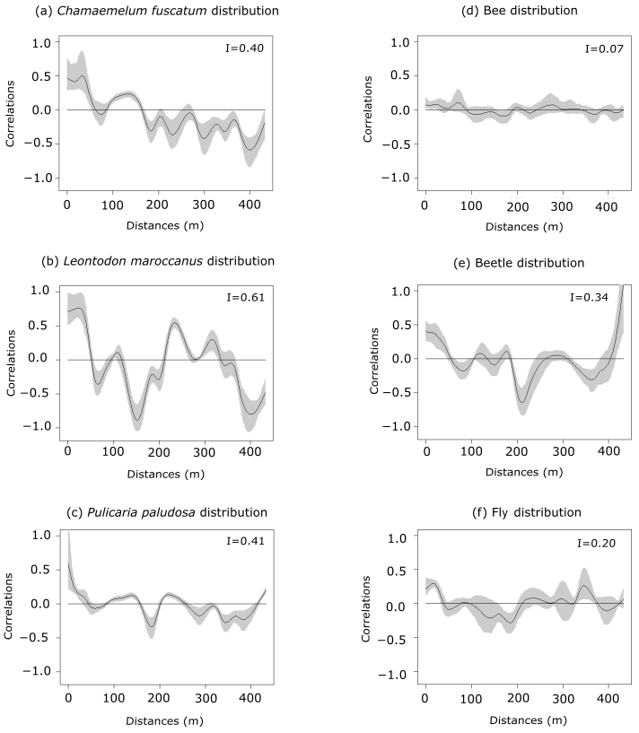
Figure 1 Spatial autocorrelation of plant abundances of the three plant species (panels a, b and c: C. fuscatum, L. maroccanus and P. paludosa, respectively) and of the three main pollinators (panels d, e and f: bees, beetles and flies, respectively) at increasing distances. The black line is the spatial correlation value that a species has for each distance; the gray shadow indicates the 95 % confidence interval. The distribution of plant species individuals is more heterogeneous than the pollinator distribution. Within each panel, Moran's I value is shown.

The three species (Fig. 1 and Table A4, Appendix A) showed a significant degree of spatial autocorrelation (Moran's I = ∼ 0.47; p value = 0.01). Generally, they were fairly aggregated at small distances, but this aggregation decayed after the first 50 or 100 m. Nonetheless, the degree of spatial aggregation of floral visitors, despite being significant, was much smaller than that of the plant species (Moran's I < 0.34; p value = 0.01; Fig. 1), especially for mobile organisms such as flies (Moran's I = 0.20) and bees (Moran's I = 0.07; p value = 0.01; Fig. 1). The reproductive success of individual plants showed a lower spatial autocorrelation for the three species compared to the plant individuals (Moran's I = ∼ 0.1; p value = 0.01; Fig. A6, Appendix A). This means that the reproductive success levels for the plants are mostly equal in relation to their spatial distribution.

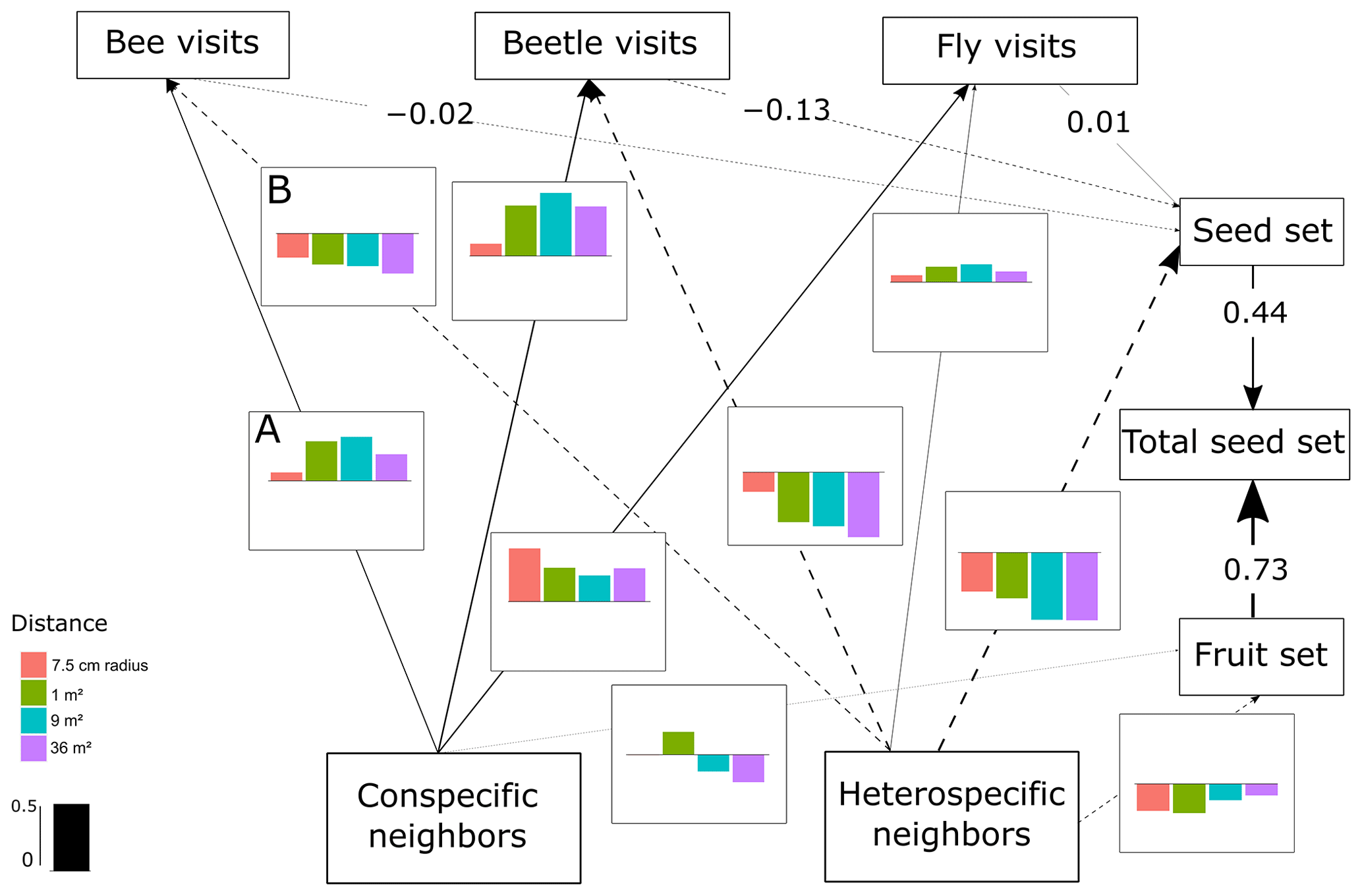
Figure 2 SEM of C. fuscatum, which includes the differences in the interactions between scales. The lines (dashed and solid lines) are proportional to the magnitude of the relationship (when different scales are relevant, we plot the mean of the standardized total effects across scales). The dashed lines are the negative relationships. When numbers are included on the paths instead of in the plot with the effect size bars across scales, it describes the standardized total effect, which remains the same across scales. The bar plots show the standardized total effects of each relationship across the different scales, and the bar in the legend represents the value of 0.5 as a visual aid. If the value of the bar plot is positive, it means that it has a positive effect, and if it is negative, it means that it has a negative effect. It is important to mention that the correlations between the variables are not visualized on the path, but in the SEM they are included (Eq. A1, Appendix A) (p value = 0.813; df = 48; R² of individual total seed set = ∼ 0.80). In this figure we include an example of how to read the figure. For example, line A indicates that the density of conspecific neighbors affects bee visits positively at all scales, while line B indicates that the density of heterospecific neighbors negatively affects bee visits at all scales.

Figure 3 SEM of L. maroccanus, which includes the differences in the interactions between scales. The lines (dashed and solid lines) are proportional to the magnitude of the relationship (when different scales are relevant, we plot the mean of the standardized total effects across scales). The dashed lines represent negative relationships. When numbers are included on the paths instead of in the plot with the effect size bars across scales, it describes the standardized total effect, which remains the same across scales. The bar plots show the standardized total effects of each relationship across the different scales, and the bar in the legend represents the value of 0.5 as a visual aid. If the value of the bar plot is positive, it means that it has a positive effect, and if it is negative, it means that it has a negative effect. It is important to mention that the correlations between the variables are not visualized on the path, but in the SEM they are included (Eq. A2, Appendix A) (p value = 0.659; df = 44; R² of individual total seed set = ∼ 0.92).

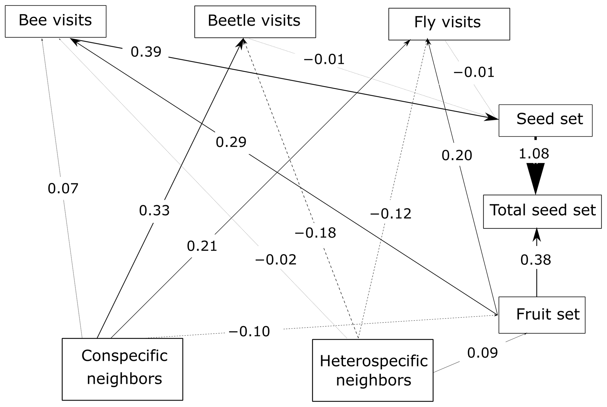
Figure 4 SEM of P. paludosa. As the ANOVA results and the AIC test suggest for this species, the unconstrained model fits the data better, and hence the scale is not considered. The lines (dashed and solid lines) are proportional to the magnitude of the relationships (we plot the standardized total effects) to exemplify the path. The numbers included on the paths are the standardized total effects, which remain the same across scales. The dashed lines represent negative relationships. It is important to mention that the correlations between the variables are not visualized on the path, but in the SEM they are included (Eq. A3, Appendix A) (p value = 0.187; df = 95; R² of individual total seed set = ∼ 0.57).

The most important finding when comparing results from the structural equation models (SEMs) was that the reproductive success of the three plant species depended on a different combination of direct and indirect paths, which indicated that there was variability in the biological strategies followed by each species. Moreover, there were two species (C. fuscatum and L. maroccanus) that were affected by the spatial scale considered and one species (P. paludosa) that was not affected by scale. The best-fitting structure of the path diagram revealed that the total number of fruits had a larger influence than the seed set on the total seed production, except in the case of P. paludosa. Comparing the direct interactions between plant neighbors (conspecific and heterospecific) and the total seed set per individual for C. fuscatum and L. maroccanus, we found a negative relation between the density of conspecific neighbors and fruit production at small scales (Figs. 2 and 3). Moreover, the effect of conspecific neighbors on the fruit set produced per individual varied depending on the scale. For both species, we saw that the effect of conspecific neighbors on fruits switched across scales. For C. fuscatum the effect of conspecific neighbors was positive at medium scales and negative at small and larger scales. Meanwhile, for L. maroccanus the effect of conspecific neighbors switched from negative to positive at increasingly larger scales. Finally for P. paludosa, the effect of conspecific neighbors on the fruit set was negative, while the effect of heterospecific neighbors was positive but weak (Fig. 4). The neighbors' (both conspecific and heterospecific) effect in the seed set (in most cases an indirect effect through pollinators) and in the fruit set was variable depending on the species. In the case of L. maroccanus there was a stronger effect of the conspecific neighbors on reproductive success due to its neighbors also affecting the seed set, and in the case of C. fuscatum the stronger effect was due to the heterospecific neighbors. The role of pollinators in these plant species was in general weak. P. paludosa, however, exemplifies the opposite pattern, in which bees had an important effect on its reproductive success, yet pollinator attraction to P. paludosa individuals depended positively on the number of flowers per individual.

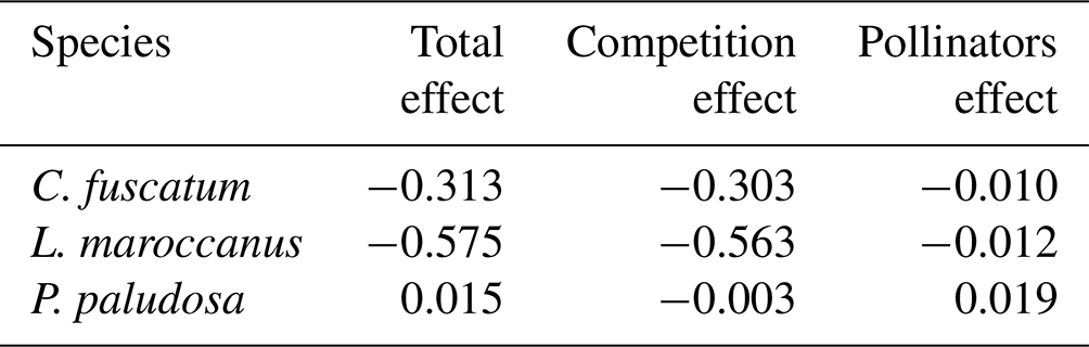
We also found a clear effect of the number of both conspecific and heterospecific neighbors on attracting pollinators. Generally, the conspecific neighbors benefited the focal species by attracting more pollinators at medium and large scales, but the effect of heterospecific neighbors was more variable. While heterospecific neighbors always affected the beetle visits negatively, they positively affected the bees in L. maroccanus and flies in C. fuscatum, but in P. paludosa there was a negative effect on the three pollinator groups. When we looked at the mean effects of the competition and pollinator-mediated paths (Table 2; see effect decomposition across scales in Table A5, Appendix A, for C. fuscatum and L. maroccanus), we observed that the positive effect of increased pollinator attraction in general only compensated for the negative effect of plant competition in P. paludosa.

Table 2 The direct effects (standardized total effects) of plant competition and the indirect effects mediated by pollinators on the plant reproductive success at the 7.5 cm radius scale (see Table A5, Appendix A, for the effects on each scale). We have chosen this scale because it is the scale most representative of plant fitness.

4 Discussion

Our most important finding is that the spatial context affects how plant–plant interactions and plant–pollinators interactions contribute to plant reproductive success. Following our main hypotheses, we observed that plants were more aggregated in space than their floral visitors, and plant–plant and plant–pollinator interactions affected in opposite ways plant reproduction success. While plant neighborhoods have a negative effect on plant reproductive success, pollinators result in a more variable but overall positive effect. However, when comparing the net effect of both sources on plant reproduction success, we found that the positive effect of pollinator visits mediated by the attraction of plant neighbors at larger scales did not compensate in general for the direct negative effect of plant local competition in two out of the three studied plants.

Following prior theoretical and observational work, we observed that plant densities, particularly those of heterospecific individuals at small spatial scales, had the strongest negative effect on plant reproductive success with negative consequences for the fruit set. We interpret this negative effect as competition for common resources such as water, nutrients or light as well as shared natural enemies (Underwood et al., 2020), yet we acknowledge that we did not explore the ultimate sources of the observed competition. Another important finding is that the scale at which competition acts was different from the scale at which pollinators were attracted. Namely, our results suggest that competition effects are stronger at smaller scales (Antonovics and Levin, 1980) and confirm that measuring neighborhoods at a 7.5 cm radius captures the strongest signal of competition (Levine and HilleRisLambers, 2009; Mayfield and Stouffer, 2017; Lanuza et al., 2018). However, distances at which pollinators are attracted remain less understood. In our case, pollinator attraction and its further positive contribution to plant reproductive success through pollination visits occur at larger scales of up to 9 m².

Indeed, the scale at which different ecological interactions are relevant might differ in other systems. Our study shows that there is a complex interplay between the intrinsic ability of plants to produce seeds in the absence of pollinators, their capacity to produce flowers and therefore to attract pollinators, and the pollinator behavior and its pollination efficacy. This is exemplified by the contrasting strategies we observed among the three studied species. For instance, L. maroccanus and C. fuscatum were not limited in the contribution of pollinators to plant reproductive success because L. maroccanus is highly self-compatible and because C. fuscatum showed no pollen limitation due to relying on a high number of visits by small flies, which ensures a large seed set across the area. In contrast, the pollination of P. paludosa was limited by the low number of bee visits needed to contribute significantly to increasing its reproductive success. This small number of visits could be due to (i) the fact that P. paludosa is a late-flowering species whose phenology mismatches the phenology of bees, (ii) the fact that P. paludosa is not a strongly aggregated species that can attract bees by itself or (iii) bees simply being scarce. Regardless of these different possibilities, our study shows that the effect of pollinators on plant reproductive success is a spatially explicit process which in turn interacts with the plant and pollinator biology. Our study shows that pollinators contribute positively to plant reproductive success, but their contribution might not be enough to compensate for the negative effects of plant competition in environments in which conspecific neighborhoods are spatially aggregated.

All plant species and pollinator guilds presented a significant pattern of spatial aggregation, although the magnitude varied greatly across species. Spatial aggregation of plant species is considered to be mediated by a combination of local dispersal and strong preferences for certain environmental conditions (e.g., water availability) (Stoll and Prati, 2001). Many annual Asteraceae species such as C. fuscatum and P. paludosa neither possess particular dispersal structures (e.g., pappus) (Howe and Smallwood, 1982; Venable and Levin, 1983) nor are attractive and big enough to be dispersed by seed dispersers such as insects or ants (Handel and Beattie, 1990; Rogers et al., 2021); therefore they tend to fall to the ground close to their mothers (Venable and Levin, 1983). Other species with pappus structures, such as L. maroccanus in this study, can be wind- or water-dispersed over long distances, and their strong spatial aggregation can be due to the selection of particular microenvironmental conditions for germination (e.g., substrate) that allow for seed germination and establishment (Venable and Levin, 1983; Nathan and Muller-Landau, 2000). For floral visitor guilds, wild bees are known to be central-place foragers that forage close to their nest (Gathman and Tscharnte, 2002), while flies instead seem to have an unspecialized pattern in which they forage distinct flowers over long distances (Inouye et al., 2015). Beetles, having a more clustered aggregation, tend to visit fewer flowers and to stay for a longer time per flower than the other guilds (Primack and Silander, 1975). These arrays of mechanisms suggest that in general spatial aggregation is more likely to be found in plants than in floral visitors. Future research could manipulate the degree of spatial aggregation of conspecific plant individuals across multiple scales to mechanistically test the relative importance of both plant–plant and plant–pollinator interactions for the reproductive success of individual plants.

Together, our study provides clear evidence that spatial aggregation across scales, from very small neighborhoods to plot scales, is key to determining the magnitude of the effect of multitrophic interactions, modulating plant reproductive success. Such correlation in conspecific individuals across scales connects pollinator attraction, and therefore the mutualistic effect of floral visits (Ghazoul, 2006; Bruninga-Socolar and Branam, 2022; de Jager et al., 2022), with the negative competitive effect of dense local neighborhoods (Albor et al., 2019; Underwood et al., 2020). This connection highlights the fact that individual reproductive success, and therefore the persistence of populations, is a matter of not only the degree of temporal autocorrelation (e.g., Lyberger et al., 2021; Martinović et al., 2021) but also the degree of spatial autocorrelation. However, the spatial effects documented here are little explored in other systems, and therefore, we point out a need to better integrate observational data with solid theory that connects plant–pollinator systems with multiple trophic interactions in a more comprehensive framework of plant population dynamics. Such integration is paramount because in our study we highlight that predicting the net effect of plant–plant and plant–pollinator interactions on plant reproductive success in spatially structured environments is complex as it results from a combination of pollinator (Underwood et al., 2020) and plant (de Jager et al., 2022) characteristics. We conclude that a more realistic understanding of the direct and indirect effects by which pollinators contribute to plant fitness needs to explicitly consider the spatial structure in which these interactions occur.

Appendix A

The following equations specified in R are the models that we use to create the SEM for each species. Equations (A1), (A2) and (A3) are equal except for some particularities for each species. The “∼” sign means that there is a relation between the predictors, and the double “∼ ∼” sign means that there is a correlation between the variables; i.e., there is a covariation. It is important to remember that fruits in our study are the same as the number of flowers.

Equation (A1). This is the model for C. fuscatum.

model C.fuscatum <- '

Plant_fitness =

seed set ~ Bee + Fly + Beetle
fruits ~ heterospecific conspecific
Bee ~ heterospecific + conspecific
Fly ~ heterospecific + conspecific
Beetle ~ heterospecific + conspecific

Individual total seed set ~ seed set + fruits

#particularities for this species
seeds ~ heterospecific
Beetle ~~ Fly
'

Equation (A2). This is the model of L. maroccanus.

model L.maroccanus <- '

Plant_fitness =

seed set ~ Fly + Beetle + Bee
fruits ~ heterospecific + conspecific
Beetle ~ heterospecific + conspecific
Fly ~ heterospecific + conspecific
Bee ~ heterospecific + conspecific

Individual total seed set ~ seeds + fruits

#particularities for this species
seed set ~ conspecific
Beetle ~ fruits
seed set ~~ individual total seed set
'

Equation (A3). This is the model for P. paludosa.

model P.paludosa <- '

Plant_fitness =

seed set ~ Fly + Bee + Beetle
fruits ~ conspecific + heterospecific
Fly ~ conspecific + heterospecific
Bee ~ heterospecific + conspecific
Beetle ~ heterospecific + conspecific

Individual total seed set ~ seed set + fruits

#particularities for this species
seed set ~~ individual total seed set
seed set ~~ fruits
Fly ~~ Bee
Fly ~~ Beetle
Fly ~ fruits
Bee ~ fruits
'

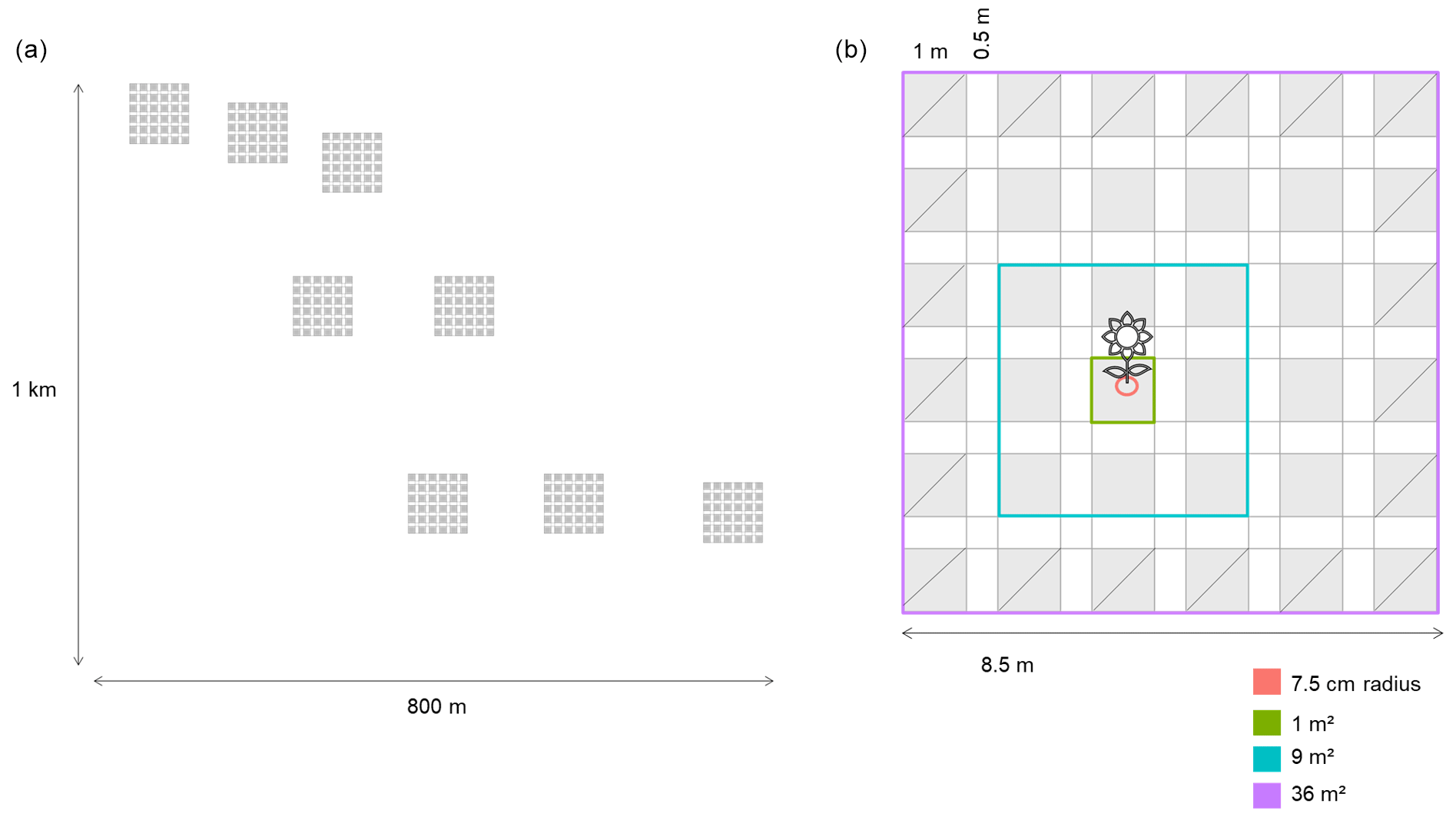
Figure A1 (a) Distribution of the eight plots across the landscape, which are distributed across an area of ∼ 1 km × 800 m. (b) Spatially explicit design of the plots located across the field. The areas with a diagonal line are the areas that have been excluded (the edges) for calculating the neighbors of a focal species, but they have been used to calculate the neighborhoods. Using this approach we get the same number of neighborhood subplots per focal species. The different colors show the different scales at which we have calculated the neighborhoods: 7.5 cm radius (0.018 m²) and 1, 9 and 36 m². Each subplot is 1 m × 1 m (1 m²), and there are 36 subplots; each subplot is separated by 0.5 m from the others.

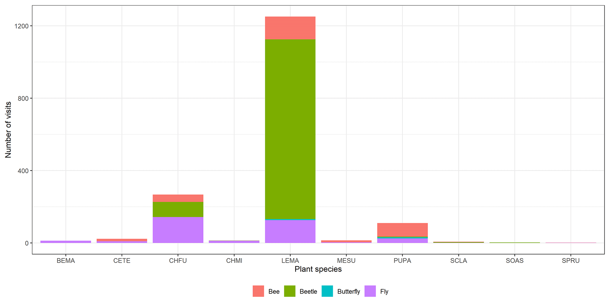
Figure A2 Floral visitor distribution across the plant species. We can observe that the most visited species are C. fuscatum, L. maroccanus and P. paludosa. C. fuscatum is visited mostly by flies; L. maroccanus is visited mostly by beetles; and lastly, P. paludosa is visited mostly by bees. See Table A1 for the plant species codes shown on the x axis.

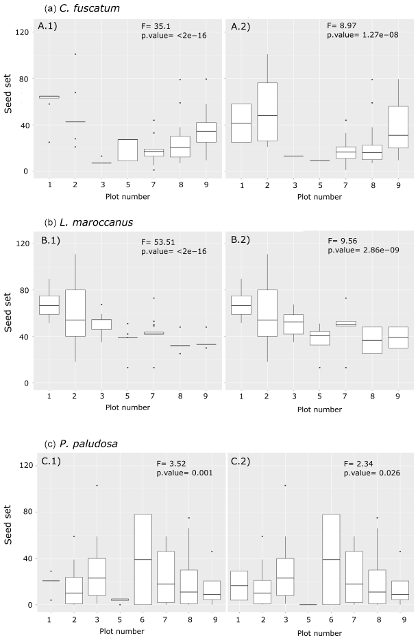
Figure A3 Differences between the number of the seed sets per individual per plot and per species (a: C. fuscatum; b: L. maroccanus; c: P. paludosa). The left column shows the seed set with the missing data that were filled with the average of the seed set per plot, while the right column shows the seed set data collected in the field. Each panel shows the F value and the p value of the ANOVA test. These results indicate that filling the missing data with the average of the plot, although not ideal, maintains the variability across plots. For a better interpretation of this figure, we have delimited the y axis to a maximum of 125 seed sets; there are four points omitted in the plot.

Table A1 List of species observed in the Caracoles estate in 2020. The code and taxonomic information of the plant species are provided. Also, the number of visits of each floral visitor group by plant species is recorded. Sample sizes represent the abundances of each species that we measured in the field, and they are correlated with their natural abundances in the site study. In these data the butterfly visits are included; however, due to the low number of visits of that group (only 13 visits), we decided to exclude these data for further analysis.

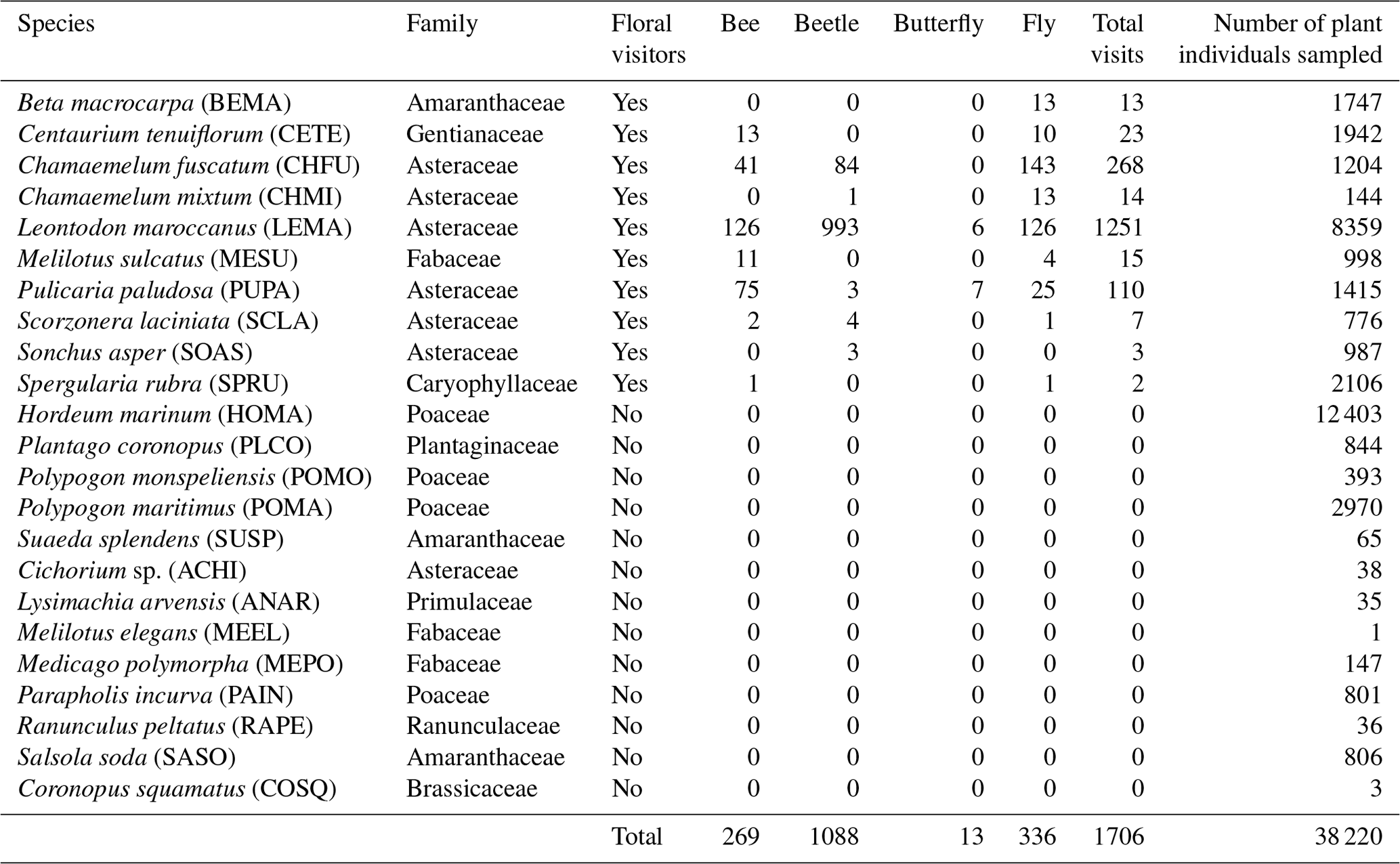
Table A2 Floral visitor frequency. The ID is the most accurate identification of the floral visitors that we have made. Each ID has the associated total number of visits recorded in the field. We classified the ID into four groups of floral visitors: bee, beetle, butterfly and fly.

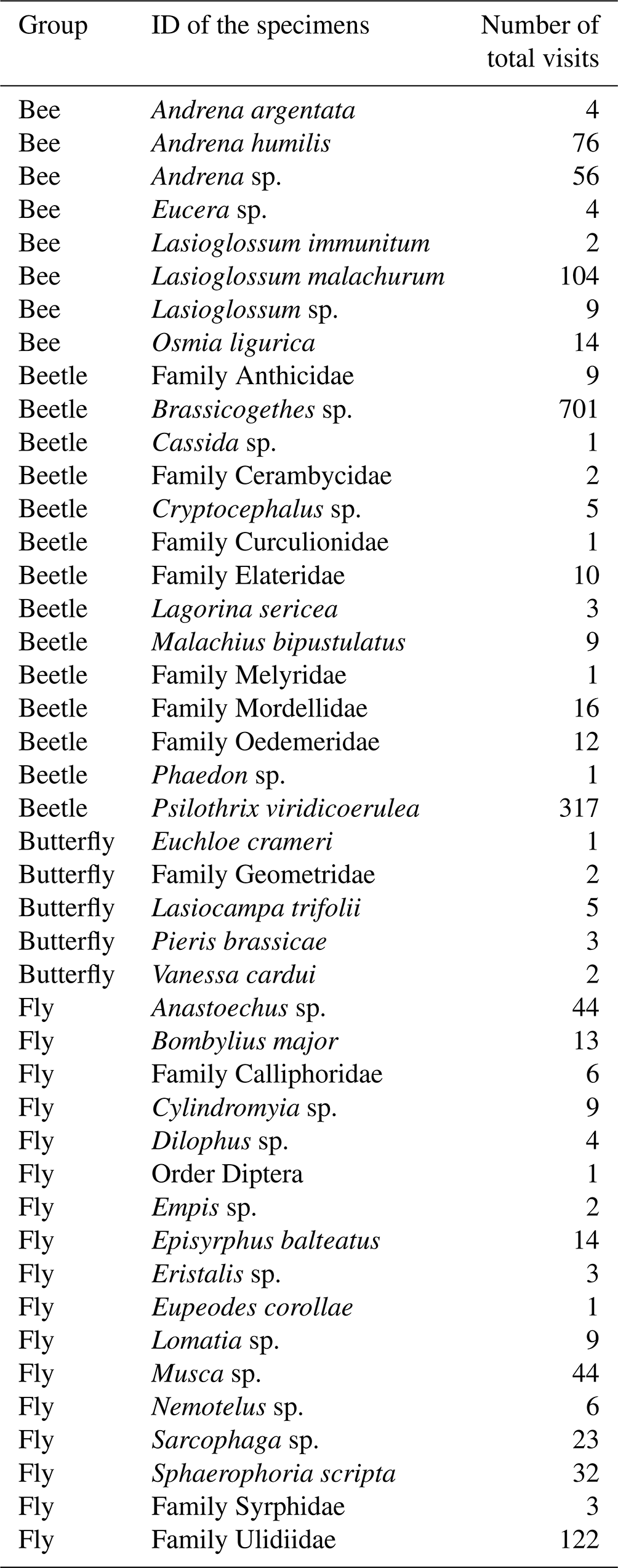
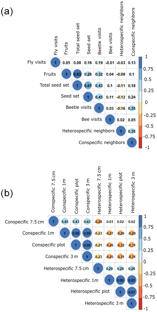
Figure A4 These plots show the correlations between the different variables. Panel (a) shows the correlations between all the variables included in the model per the three species. The total seed set data shown are per plant individual. Panel (b) shows the correlations between the different scales of neighbors (7.5 cm radius and 1, 9 and 36 m², plot level). The dark colors of the cells indicate that there is a strong correlation, and the light colors mean the opposite – there is a slight correlation.

Table A3 ANOVA results for each plant species for both the constrained and the multigroup model. This allows for checking if the models should include the spatial scale (multigroup models) or not (constrained models). For each species, we selected the model with the lowest AIC and tested if models differ using an ANOVA. The “^∗” symbol means that the ANOVA is significant, which implies that both models are different. In the case of C. fuscatum and L. maroccanus, the models that are more parsimonious (lower AIC) are the multigroup model, and in the case of P. paludosa, the most parsimonious model is the constrained model. BIC denotes the Bayesian information criterion.

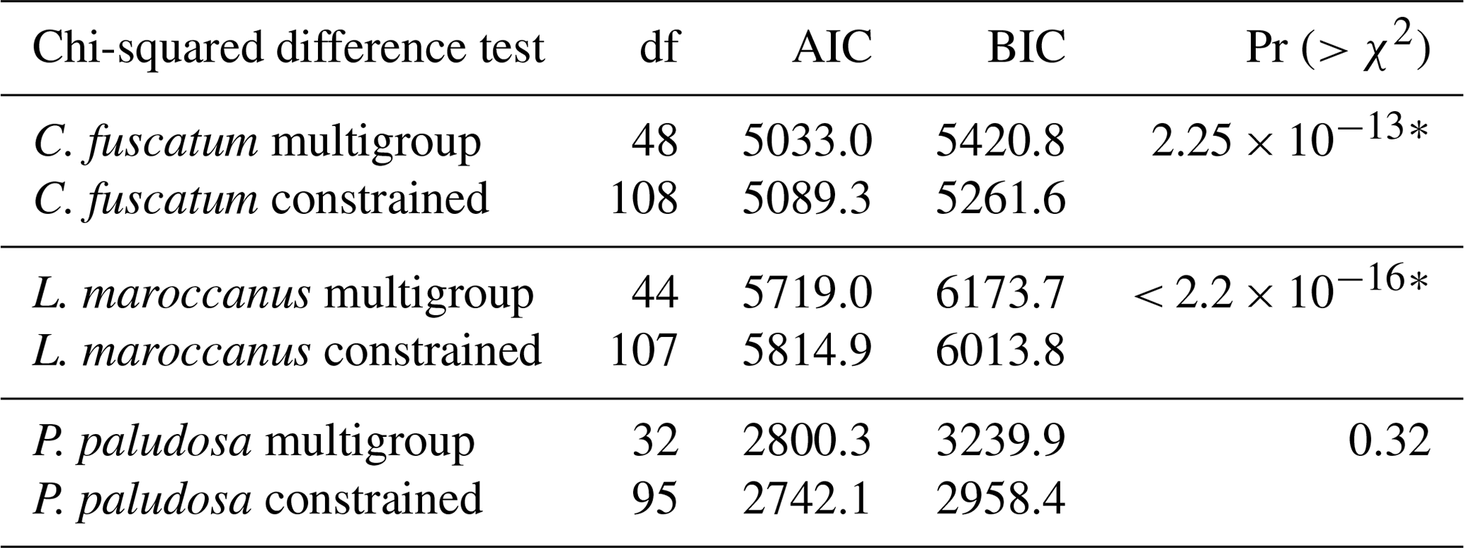
Table A4 Summary of the most relevant characteristics (flowering season, principal pollinators, dependence of pollinators and the aggregation level of conspecific plant individuals) of the three main plant species: Chamaemelum fuscatum, Leontodon maroccanus and Pulicaria paludosa.

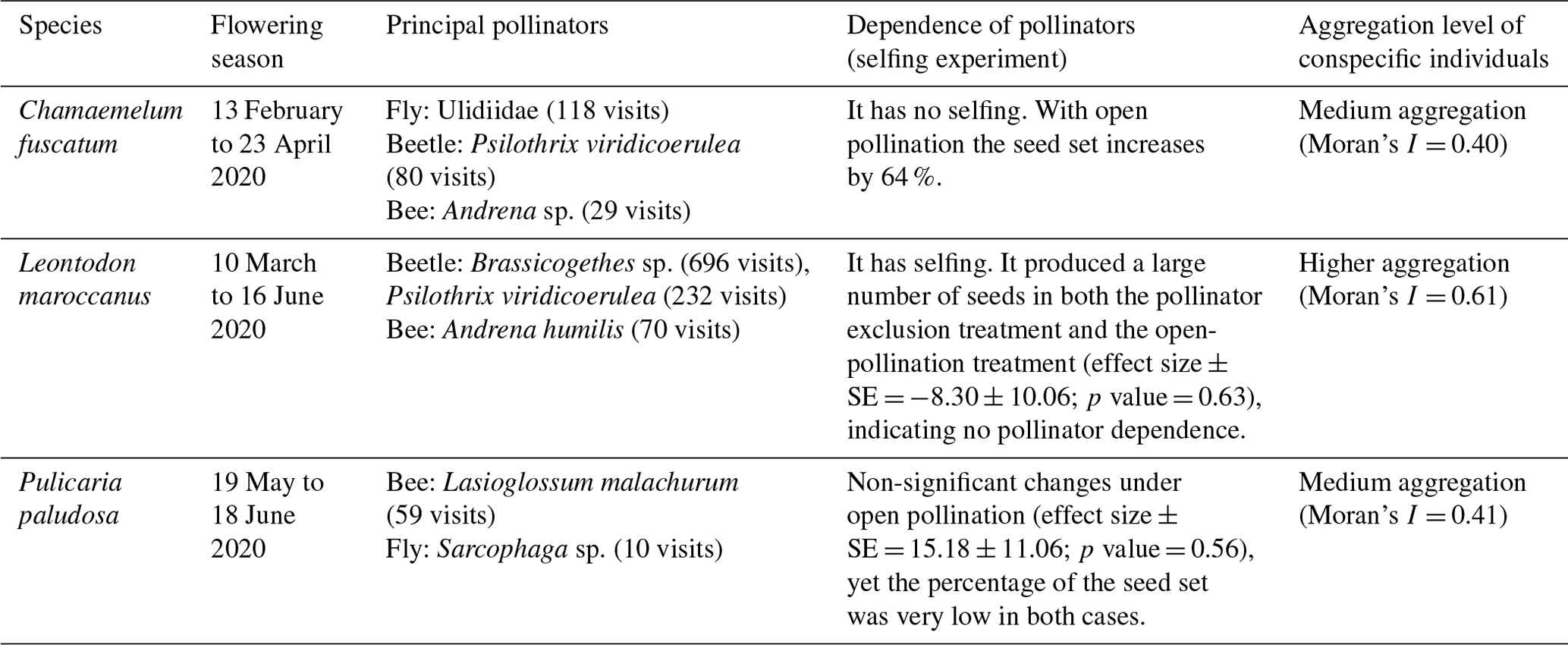
Table A5 Decomposition of the direct and indirect effects across the different scales in the species that are scale dependent (C. fuscatum and L. maroccanus). The standardized total effects are shown.

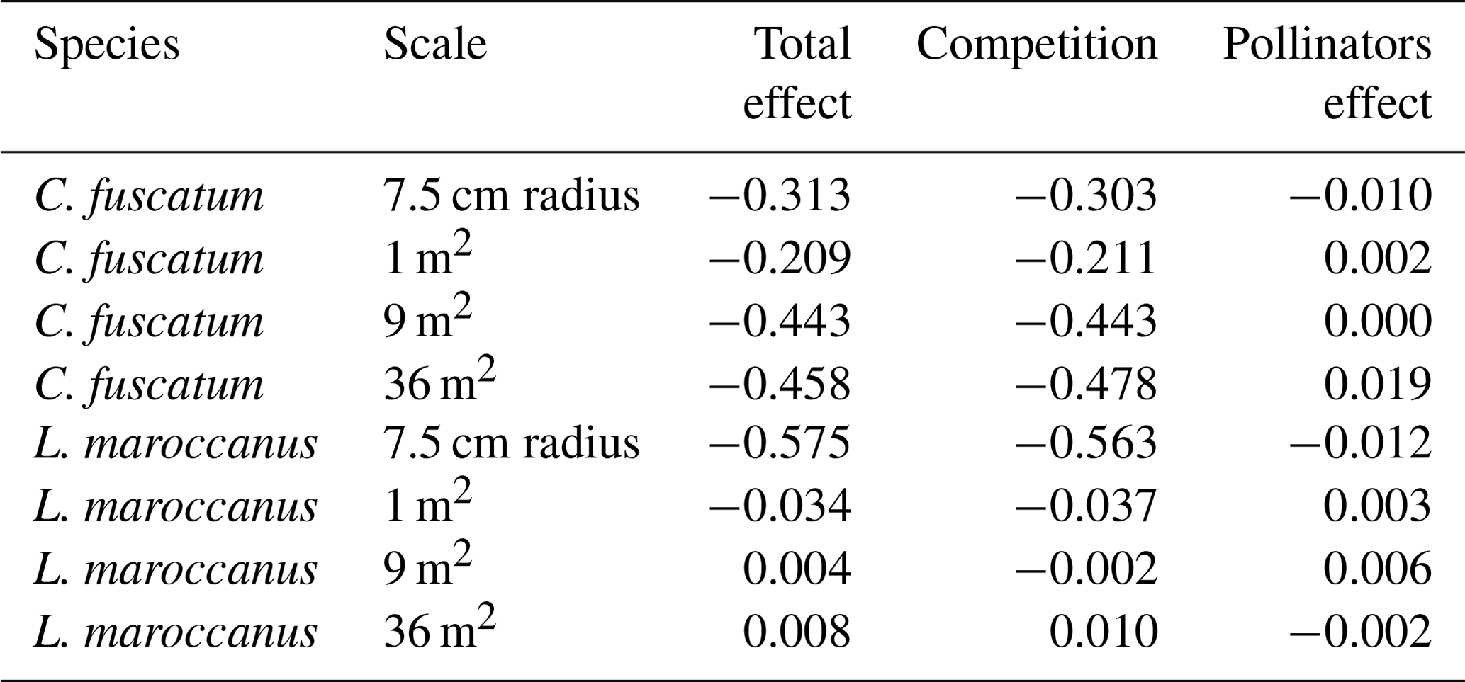
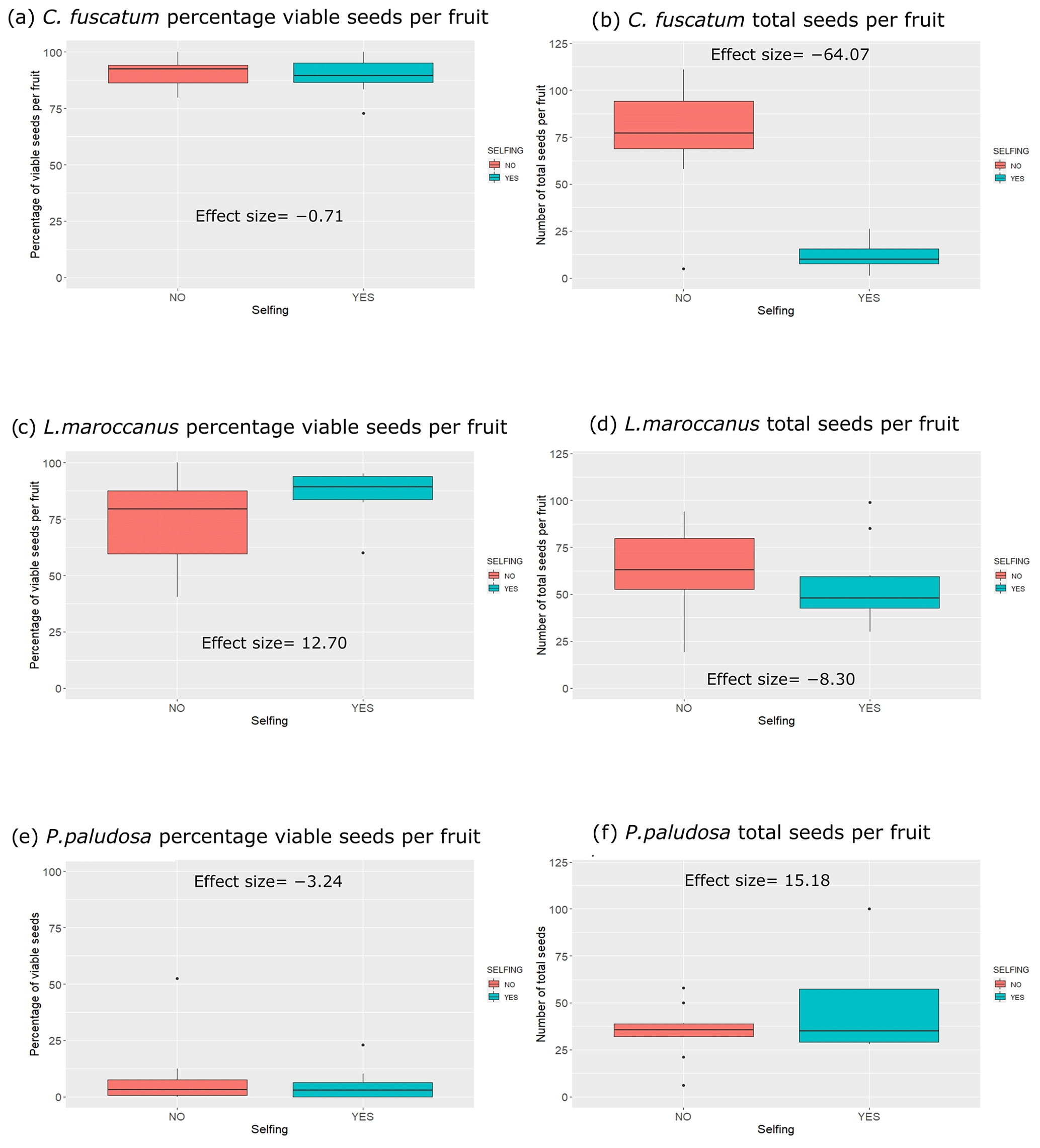
Figure A5 Differences for each plant species considering the seed set and the individual total seed set of the selfing experiment (with or without pollination). In the left column of the plots, we have the percentage of individual total seed sets per species per treatment, and in the right column we have the number of total seeds (viable and not viable seeds) per species and per treatment. The numbers that appear inside the plot are the effect sizes.

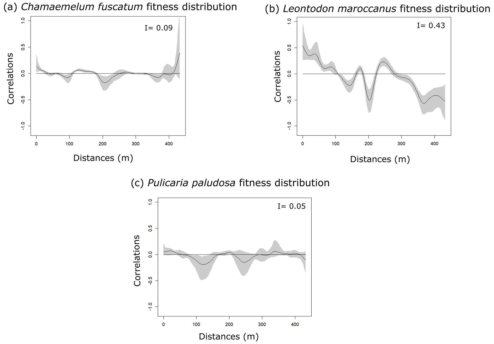
Figure A6 Spatial autocorrelation of fitness (individual total seed set) distribution of plant species. The black line is the spatial correlation value that a species has for each distance; the gray shadow indicates the 95 % confidence interval. The I values are the result of Moran's I statistic.