Pollination supply models from a local to global scale

Ecological intensification has been embraced with great interest by the academic sector but is still rarely taken up by farmers because monitoring the state of different ecological functions is not straightforward. Modelling tools can represent a more accessible alternative of measuring ecological functions, which could help promote their use amongst farmers and other decision-makers. In the case of crop pollination, modelling has traditionally followed either a mechanistic or a data-driven approach. Mechanistic models simulate the habitat preferences and foraging behaviour of pollinators, while data-driven models associate georeferenced variables with real observations. Here, we test these two approaches to predict pollination supply and validate these predictions using data from a newly released global dataset on pollinator visitation rates to different crops. We use one of the most extensively used models for the mechanistic approach, while for the data-driven approach, we select from among a comprehensive set of state-of-the-art machine-learning models. Moreover, we explore a mixed approach, where data-derived inputs, rather than expert assessment, inform the mechanistic model. We find that, at a global scale, machine-learning models work best, offering a rank correlation coefficient between predictions and observations of pollinator visitation rates of 0.56. In turn, the mechanistic model works moderately well at a global scale for wild bees other than bumblebees. Biomes characterized by temperate or Mediterranean forests show a better agreement between mechanistic model predictions and observations, probably due to more comprehensive ecological knowledge and therefore better parameterization of input variables for these biomes. This study highlights the challenges of transferring input variables across multiple biomes, as expected given the different composition of species in different biomes. Our results provide clear guidance on which pollination supply models perform best at different spatial scales – the first step towards bridging the stakeholder–academia gap in modelling ecosystem service delivery under ecological intensification.

1 Introduction

Agricultural intensification enabled a dramatic increase in agricultural production during the second half of the 20th century, with a growth rate even exceeding the population growth rate (Wik et al., 2008). However, the last 2 decades have witnessed a saturation in the yield of major crops in some countries (Grassini et al., 2013). Given expected population growth and associated increases in the demand for agricultural products, the pressure to expand agricultural areas will increase in many regions (Foley et al., 2011). Short-term food production can be increased to a certain extent if such expansion occurs and conventional agricultural intensification practices are applied to currently underperforming lands. Nonetheless, in the long run, these land-use practices come at the cost of massive environmental damage, undermining the capacity of ecosystems to sustain food production and other ecosystem services (Foley, 2005), which would make agricultural intensification ineffective, if not detrimental.

One way to reduce the environmental impact of conventional agricultural intensification while keeping productivity near optimal values is to use ecological intensification (Bommarco et al., 2013), which relies on nature-based solutions to enhance crop productivity. These ecological-intensification practices can potentially avoid much of the environmental damage associated with the future increase in food demand (or even, in the best-case scenario, drive the recovery of already-damaged ecosystems). As such, the ecological-intensification approach has attracted the scientific community's attention, and the scientific community, in turn, has provided evidence of its potentiality (Cassman et al., 2010; Bommarco et al., 2013; Kovács-Hostyánszki et al., 2017).

Pollination services are a paradigmatic example that illustrate the ability of ecological intensification to enhance crop yield because the yield of more than 70 % of the crops grown worldwide depends, to some extent, on animal pollination (Klein et al., 2007). Furthermore, pollination contributes to around 10 % of the global value of agriculture (Lautenbach et al., 2012). During the last few decades, the proportion of cropland devoted to pollinator-dependent crops has been increasing (Aizen et al., 2008). However, common practices of conventional intensification (e.g. high input of pesticides and fertilizers, landscape simplification, limited crop rotation) are harmful to pollinators (Le Féon et al., 2010; Aizen et al., 2019) and therefore counter-productive for pollinator-dependent crops. Climate change may exacerbate the problem, shifting the location of pollinator-dependent crops from areas with high pollinator availability to less suitable landscapes (Polce et al., 2014). To address the shortage of wild pollinators, some farmers locate honeybee colonies near their fields, but the service provided by honeybees alone is often lower than when wild pollinators are also present (Klein et al., 2003; Greenleaf and Kremen, 2006; Garibaldi et al., 2013; Kennedy et al., 2013). Thus, enhancing wild pollinator populations opens up the possibility of a win–win situation where ecological intensification leads to higher yield while enhancing ecosystem functioning and biodiversity (Garibaldi et al., 2016; Dainese et al., 2019; Woodcock et al., 2019). Yet, as opposed to the use of managed honeybees and other inputs which can be easily tracked by farmers, understanding the availability of wild pollinators and the pollination services they can provide is complex. One effective way to facilitate bringing this knowledge to the interested stakeholders is by using modelling approaches (Polce et al., 2013).

Pollination service models can compute metrics like pollinator visitation rates or other proxies for pollinator benefits within a particular geographic area to improve pollination management. The visitation rate of wild species is positively correlated to pollination services like fruit set and pollen deposition (Garibaldi et al., 2013; Rader et al., 2015; Dainese et al., 2019). Farmers can use predictions to optimize pollination services in the fields, and policy-makers can develop effective agri-environmental schemes or promote governmental initiatives for conservation such as the EU Pollinators Initiative (Zulian et al., 2013; European Commission Joint Research Centre, 2018) or the US Pollinator Research Action Plan (The White House, 2015). The importance of describing landscape suitability for pollinators is clear from an economic and ecological perspective. Whereas there is a certain consensus on some general statements, for example, the availability of natural and semi-natural habitats are beneficial for most pollinators (Garibaldi et al., 2011; Klein et al., 2012), there is an incomplete understanding of the habitat conditions and mechanisms that allow for the presence of particular species at particular locations (Jha and Kremen, 2012; Rogers et al., 2014; Leong et al., 2014; Dicks et al., 2015).

Several modelling approaches have been used in the past to predict pollinator abundances. On the one hand, mechanistic or process-based (Lonsdorf et al., 2009; Olsson and Bolin, 2014; Häussler et al., 2017; Everaars et al., 2018) and agent-based (Becher et al., 2014, 2018) models describe, with varying degrees of complexity, mechanisms that characterize the behaviour of pollinators. The final output of these models is always a consequence of the mechanisms that guide individual pollinator behaviours. As such, they can provide detailed output on ecological processes, such as pollinator nesting or foraging preferences, which aids the interpretability of results. However, these models require considerable ecological knowledge as input, which may be inaccurate and biased (Gardner et al., 2020).

An alternative is to use data-informed ecological inputs (Gardner et al., 2020) or purely data-driven models like species distribution models (Polce et al., 2013, 2018) and machine-learning approaches (Kammerer et al., 2021). Data-driven models to predict species distributions form the basis of these data-driven models used to infer the relationships between environmental conditions and the target variable (typically occurrence), enabling the computation of predictions at unobserved locations. As opposed to mechanistic models, data-driven models depend on a training process, which implies that they typically require a large number of data and that predictions can only be made using the same variables (with the same pre-processing) as the ones used in the training. Moreover, the target variable depends directly on the dataset used. Statistical methods usually rely on a mixture of systematic surveys and citizens' observations that are not specifically attached to crop fields, which means that they predict occurrence rather than the crop visitation rate. Finally, despite theoretical knowledge of biological processes being important for the development of data-driven models (e.g. for the selection of variables), they ultimately depend on data rather than theory. In that sense, data-driven models are phenomenological, and, as such, they cannot be generalized to scenarios not represented in the input dataset.

Regardless of the modelling approach adopted, ecological-intensification and pollination service models should also address the needs of the end users. For instance, growers need to balance their pollination needs with their wider farming practices (Kleijn et al., 2019) whilst considering costs and whether they are subject to subsidies (Osterman et al., 2021). Thus, highly parameterized models might be difficult to apply if the necessary inputs require a considerable amount of time to be estimated. In that regard, the data inputs for some mechanistic models (MMs hereafter; e.g. Lonsdorf et al., 2009) are publicly available datasets (see Sect. 2.1.1). Additionally, machine-learning (ML hereafter) models can also run on global datasets that are ready to use in public repositories. Hence, both the MMs and the ML models, once implemented, can be easily fed with data from any region worldwide. This property makes them highly applicable and transferable among regions.

The geographic scale of the assessment is key because it differs depending on the stakeholder. Growers might be interested in ranking locations regarding their potential pollination service within a particular area of interest, while landscape managers or policy-makers may want to target policy interventions for maximum ecological gain over a much wider geographic extent. In general, each user is interested in knowing, at the scale of interest, the following: first, whether there is one or more pollination service models that provide reliable results. Second, whether these models are able to quantify the reliability of their results. Finally, in the case that there are models that provide results with a satisfactory reliability, a hypothetical stakeholder would be interested in knowing which one is more reliable. All in all, any exercise that enables a deeper understanding of the potentialities and limitations of different modelling approaches, such as the one presented here, may be important to answer these questions.

Here, we use publicly available datasets extracted from the Earth Engine Data Catalog (Gorelick et al., 2017) to evaluate the ability of three types of pollination service models (MM, ML and data-informed MM (DI-MM)) to correctly rank sites according to their pollination service supply at three different geographic levels (local, biome and global). We then validate these results using a recently published global database on crop pollination (CropPol; Allen-Perkins et al., 2022). We also derive the importance of several factors in the observed visitation rate of pollinators, including environmental variables, landscape properties and human–ecosystem interactions.

2 Materials and methods

2.1 Modelling approaches

We used three different modelling approaches to predict pollinator services to crops and used a publicly available dataset to validate the results of the three approaches. Specifically, we used CropPol (Allen-Perkins et al., 2022), a global, dynamic and open database with information collected at 3022 agricultural sites with defined coordinates (see Fig. D1). It compiles georeferenced information from 202 studies focused on crop pollination, each with multiple geolocated field measurements. Such information includes the abundance of pollinators (separated by taxonomical group), pollinator richness, crop variety or management practices, among other features. Sampling methods include transects, using sweep nets and focal observations. Records from studies that use pan traps have been ruled out because pan traps attract insects and, as such, bias the measurements obtained with this methodology towards higher values compared to other methods (Portman et al., 2020).

2.1.1 The mechanistic model

We base the MM on a model developed by Lonsdorf et al. (2009), widely used in the ecosystem service literature (Zulian et al., 2013; Sharp et al., 2018). The model's output is a dimensionless score (with values ranging from 0 to 1) that describes the expected rate of pollinator visits to a given location. It uses the nesting and foraging suitability of the landscape for pollinators, calculated using experts' assessment and land cover maps, expressed in the form of lookup tables that link land cover types with the availability of floral and nesting resources. On top of that, the typical flight distance is used to define the areas that are within the foraging range of the pollinators (with a weight that decays with the distance using a Gaussian decay function). The typical flight distance is used here as a synonym for the typical homing distance defined by Greenleaf et al. (2007), i.e. the distance at which 50 % of the individuals cannot return to their nest.

We extracted land cover layers from Collection 3 of the Copernicus Global Land Service Land Cover layers (CGLS-LC100; Buchhorn et al., 2020). This collection has important advantages. First, it is globally available. Second, it has a moderately high spatial resolution of 100 m. The spatial resolution is several times lower than the typical flight distance used for bumblebees and other wild bees (30 and 5 times lower than the typical flight distances considered in this work, respectively), and therefore it is appropriate for this study. Third, it offers not only discrete classes of land cover type, but also continuous layers that estimate the cover fraction of nine basic land cover types, such as shrubland and cropland (see Table E1). This feature is significant, since it allows us to combine the scores of several land cover types in every pixel with a weight that corresponds to the cover fraction of each land cover type. Fourth, it has been updated yearly since 2015. Thus, we can use the version of the land cover map corresponding to the sampling year in the CropPol dataset, for observations registered in 2015 or later (40 % of the observations used). Observations before 2015 are validated using the 2015 land cover map. Tree canopy cover is extracted from the Global Forest Cover Change (GFCC) Tree Cover Multi-Year Global 30 m dataset (Sexton et al., 2013).

Despite the advantages of the land cover maps used in this work, we also note some drawbacks. In particular, the thematic resolution is relatively coarse. In the continuous land cover map, all forest types are included in the category tree. The discrete land cover map classification is more comprehensive regarding forests, including 12 different subtypes (see Table E2), but it does not include other fine-scale habitats, such as hedgerows, or distinguish between other subtypes like improved versus semi-natural grasslands. In general, the thematic resolution determines the level of detail that can be incorporated into the input tables of the MM and DI-MM, and this resolution is moderately low. Moreover, the 100 m spatial resolution implies that any difference in habitat configuration at a scale < 100 m would not be taken into account.

The MM is based on the assumption that the abundance of pollinators is driven by the quality of resources for foraging and nesting. To assess the availability of those resources, Lonsdorf et al. (2009) propose the use of lookup tables, which can be used to remap land cover types into scores for nesting and floral resources' quality. Quantitative field estimates can derive nesting and floral resource values, but commonly they are derived from expert opinion. Ideally, input information includes different seasons, different geographic areas or biomes, and many pollinator species (or functional/taxonomical groups). For all the studies covered in this work, such a level of detail is difficult to achieve. Thus, we tested the performance of two different tables of floral and nesting suitability across different land cover types based on expert opinion. First, we used the coordinated assessment of three leading experts in ecology (Ignasi Bartomeus, Francisco de Paula Molina and Ainhoa Magrach), who based the scores on their extensive experience and the values obtained by the global assessment by Alejandre et al. (2023) for several basic land cover types. We apply the lookup table to a land cover map with continuous fields (each pixel describes the percentage of each land cover type; see Table E1). Second, we used an adaptation of the tables used by the Joint Research Centre (JRC) ESTIMAP (Zulian et al., 2013) to the land cover types used in this work. We apply the lookup table to a land cover map with discrete fields (each pixel corresponds to one land cover type) but with more land cover types than in the first approach (for example, distinguishing broadleaf and needleleaf forests, Table E2). The first approach (Table E1) has the advantage of considering more than one land cover type per pixel, weighing the scores based on the percentage of the pixel (100 × 100 m) covered by each land cover type. Nevertheless, thematic accuracy is higher for the second approach (Table E2).

We classified pollinators according to CropPol into two taxonomical groups, bumblebees (genus Bombus) and all other wild bees, and computed MM scores for each taxonomic group separately. We set a typical flight distance for each taxonomical group based on the intertegular span registered in Traitbase (Kendall et al., 2019; Traitbase, 2023), which includes records from species in Europe, North America and Central America, Australia, and Asia, and the parameters found by Greenleaf et al. (2007). We used records in Traitbase from the species represented in the genus Bombus to compute the typical flight distance for the bumblebee model and from the species belonging to the remaining genus for the other wild bees model. The values, in metres, were in the ranges [913, 4932] and [0, 5444] for bumblebees and other wild bees, respectively. The mean values were 2974 and 619 m, respectively, which were rounded to 3000 and 500 m (see Table E4). Despite the wide range of possible flight distance values, we think that, using 3000 and 500 m, we represent the foraging behaviour of long-range foragers (bumblebees) versus short-range foragers (other wild bees) well. The maximum flight distance was set to 2 times the typical distance. We did not consider Apis species because their abundance depends on human management rather than landscape properties, nor did we consider syrphid flies because they are not central-place foragers – a central assumption of MM modelling. Therefore, wherever pollination services are provided fundamentally by species other than bumblebees or other wild bees, the models presented here cannot be applied directly.

In addition, we included several new components to test whether they improve the predictive capacity of the original model by Lonsdorf et al. (2009) (see Appendix A). These include the impact of landscape elements such as forest edges, forest openness, crop field size, land cover diversity and distance to semi-natural land, plus an additional component to model pollinator activity based on temperature and solar radiation (Zulian et al., 2013). Moreover, in order to reward to some extent those places where organic farming is practised, we increased the score of some land cover types by 0.1 when evaluating the model in organic farms. This increase was set arbitrarily, but it is similar to the one applied by Zulian et al. (2013) for the same concept. Management practices are extracted directly from CropPol.

2.1.2 The data-informed mechanistic model

The DI-MM is essentially the same as the MM approach but uses a different input table (Table E3), calibrated as follows. Instead of expert opinion, we used genetic algorithms (GAs) with the help of the R package GA version 3.2.2 (Scrucca, 2013, 2017) to find the input values that maximized the rank correlation in a subset of the CropPol data (the training dataset; see Sect. 2.2). Because of the need for training data, the DI-MM was not evaluated using the entire CropPol dataset but only the test set, which is totally independent of the training set. We computed a population size equal to 400 table values and iterated through 150 generations. For each table computed in every generation, we calculated Spearman's rank correlation coefficient between the observed visitation rate of the training sites and the DI-MM score. The 20 tables (5 %) with the highest rank correlation coefficient in the training data, using a 5-fold cross-validation process, were selected in every generation. The floral scores for land cover types snow and water, as well as the nesting score for snow, were forced to 0. The floral and nesting scores for the remaining land cover types were free to vary from 0 to 1. Finally, the DI-MM output was computed using the MM with the calibrated lookup table (Table E3), applied over a land cover map with continuous fields.

2.1.3 Machine-learning models

We used scikit-learn 0.24.1 (Pedregosa et al., 2011) for the ML models. We extracted the candidate predictors for the ML model by combining different data sources related to landscape, soil properties, climate, topography, energy balance, water balance, ecological regions and human–ecosystem interactions (see Table F1 and Appendix B).

After the preparation of the input data and subsequent split into training and test datasets (Sect. 2.2), we set apart the test data subset and evaluated the 55 possible estimators of the type regressor available in the software package. Regressors, in contrast to classifiers, are models that can be trained to predict a continuous variable, for example the crop visitation rate, as in the present case. For the selection of the best candidates, we trained the 55 available estimators with default parameters using the training set. The three estimators that showed the best performance, in terms of showing lower mean absolute error (MAE), were as follows: the support vector regressor (SVR), Bayesian ridge (BayR) and gradient boosting regressor (GBR). We did not select only one option in order to compare results of different types of ML models too.

We explored the hyperparameter space in these three estimators and chose the best hyperparameters via a cross-validated random search within a plausible interval of input parameters using the training set (using the function RandomizedSearchCV in scikit-learn). ML predictions were computed in the test set using those estimators individually, with the best set of hyperparameters for each of them.

While the MM and the DI-MM outputs provide dimensionless scores between 0 and 1 as a proxy for the predicted crop visitation rate, the ML models' output is a value of the predicted crop visitation rate and an estimation of the importance of each predictor in the models. Further, although in the case of the MM and DI-MM approaches we were able to provide different inputs for bumblebees and other wild bees separately, the number of input data is especially critical for the ML models. Thus, we evaluated the ML models using the data for bumblebees and other wild bees combined; i.e. the number of bumblebee observations was added to the number of other wild-bee observations.

The computation of feature importance depends on the specific ML model used. For the GBR, the computation of feature importance is performed based on the impurity of the tree at the nodes. A GBR is an ensemble model based on the combination of results from different decision trees. In decision trees, a tree-like model is built, and each node represents a condition based on a particular variable. The condition is used to split the tree into new branches with the possible outcomes of the decision. The nodes at the end of the branches are the leaf nodes that represent the output of the model. The impurity is a measurement of how mixed the instances are regarding the target variable. The goal of splitting branches in the decision tree is to reduce impurity in the nodes as much as possible. Impurity-based feature importance gives importance to features according to how much they contribute to decreasing impurity. For the BayR and SVR models, the feature importance is computed using the permutation importance technique. This technique consists of computing how much the model's performance decreases when the values from a particular feature are replaced by random values. The larger the decrease in the model's performance, the larger the importance assigned to the feature. In both cases (impurity-based and permutation importance), the values computed for every feature are normalized so that the sum is equal to 1.

2.2 Model validation

We validated the results of our three modelling approaches at three different spatial scales: global, biome (see Table G1 for the list of biomes included) and local scales. For the analyses that included records from different studies (analyses at the biome and global scales), we harmonized the measurements of pollinator abundance. We transformed the measurements of abundance into visitation rate (counts per minute) using the total sampled time, and we expressed the values on a natural logarithmic scale:

$$\begin{array}{}\text{(1)}& \ln \left(V_{\mathrm{obs}}\right)=\ln \left({\displaystyle \frac{\mathrm{abundance}+\mathrm{1}}{\mathrm{total}\mathrm{sampled}\mathrm{time}}}\right).\end{array}$$

The visitation rate (visits recorded per minute) is a metric commonly used in pollination studies (see, for example, Garibaldi et al., 2013; Burkle et al., 2013; Rader et al., 2015) as a proxy for the overall number of pollinator visits received, which is directly linked to the reproductive success of plants. The comprehensive study by Garibaldi et al. (2013) in 41 crop systems shows that such correlations are moderate, with a mean Pearson’s correlation coefficient of 0.28 with fruit set and 0.39 with pollen deposition.

We filtered the records present in CropPol to ensure its completeness and coherence for the analyses (see Appendix C). Moreover, for the models that require training (ML models and DI-MM), it was necessary to split the set of records into training and test subsets.

The set of records used in the DI-MM and ML models consists of 1007 records, which were split into training (790 records, 78 %) and test (217 records, 22 %) subsets. In general, the training set should be large enough to enable appropriate training of the models, while the test set should be large enough to enable the appropriate evaluation of the models. Inevitably there is a trade-off between the two, and the ideal percentage depends on the availability of data and the specific application. Percentages of around 80 % and 20 % are typical in ML (Géron, 2017), which is in line with the percentages used here. We used the training set to calibrate the tables in the DI-MM and at every step of the ML pipeline: collinearity analysis, model selection, hyperparameter tuning and computation of feature importance. The test data were set apart at the beginning of the analyses and only used for the computation of predictions, which is considered best practice to avoid any bias (Géron, 2017). Note that this implies that the ML model and the DI-MM results are reported for the sites of the test set, while the results of the other MMs are reported for the entire dataset because they do not require any training subset for the computation of the scores.

Given that observed abundances in the same study area are, most likely, highly correlated, our random splits were based on the author identifiers because a single author may conduct different studies in the same area over different years or crops. Hence, predictions were made on unseen study areas. At the same time, we wanted the training set to represent the range of biomes present in the database. Hence, the random split was stratified to preserve the proportional number of records in every biome.

We performed the selection of the best-performing ML models and their hyperparameter tuning using 5-fold cross-validation in the training set. In this case, the scarcity of data prevented us from using an author identifier to create the five subsets. Instead, the random split for cross-validation was based on the study identifier and stratified by biome.

2.3 Metrics

Finally, we assessed the quality of the predictions from the models based on the observed rank correlation with observations, using Spearman's coefficient (S_ρ). S_ρ allows us to evaluate whether there is a monotonic relationship between scores and the observed visitation rate, regardless of the model type. This is important in this study because it is a legitimate way to compare models that provide outputs in different units (the MM and DI-MM give a dimensionless score, while the ML models give predictions about the visitation rate). In addition, these results are interesting for stakeholders, as they are relative only to the specific study sites. This aspect becomes valuable in supporting initiatives that rely on comparing the performance of different sites within an area of interest. For instance, the findings can be used to prioritize the restoration of the worst-performing areas or to determine optimal locations for crop cultivation.

In addition to S_ρ, in order to enable the direct comparison with other studies using different metrics, we also show the coefficient of determination r², the MAE and the root-mean-square error (RMSE).

3 Results

3.1 Global scale

At a global scale, the MM, DI-MM and ML models show contrasting results for all metrics used to evaluate their predictions. In Table 1, we show the results obtained for every model tested at a global scale. The MM is only tested for the taxonomical group of other wild bees (see explanation below in this subsection), under different configurations. The configurations correspond to the activation of the additional modules (pollinator activity, open forest, etc.) implemented in the MM (see more details in Appendix A). The configurations considered for the MM execution are as follows: every module activated (configuration all modules), every module deactivated (configuration baseline) or modules activated one by one.

Table 1 Metrics obtained comparing predictions and observations from different models, at a global scale: coefficient of determination (r²), Spearman's coefficient (S_ρ), mean absolute error (MAE) and root-mean-square error (RMSE). The MM is tested for the taxonomical group of other wild bees at a global scale under different configurations, i.e. activating different modules one by one: pollinator activity, open forest, etc. Test results of the baseline (no additional module) and all modules (every module activated) configurations are also reported. The ML models (GBR, SVR and BayR) are applied to the combined data from the two taxonomical groups together. Here (and later in the text), “LC” denotes land cover, “landsc.” denotes landscape and “dist.” denotes distance.

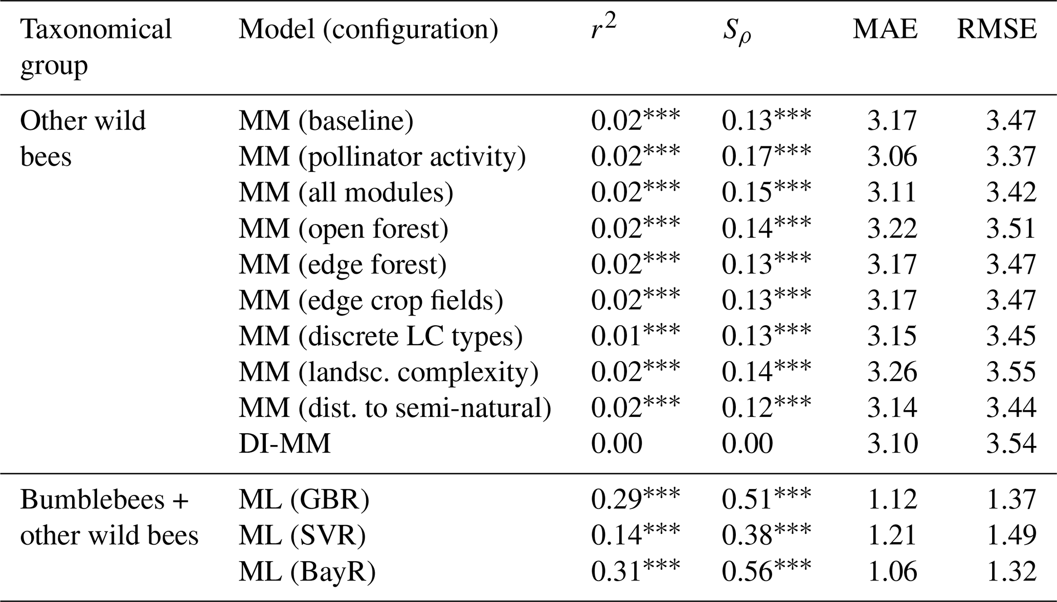
^∗ p value < 0.05. ${}^{\ast \ast }$ p value < 0.01. ${}^{\ast \ast \ast }$ p value < 0.001.

The MM (in every tested configuration) shows a moderate and positive rank correlation for the group of wild bees other than bumblebees ($S_{\mathit{\rho }}\in [\mathrm{0.12},\mathrm{0.17}]$). Adding the new components to the baseline model improved the agreement between observed and predicted values. In particular, the module of pollinator activity based on temperature and solar radiation increased the rank correlation for other wild bees at the global level, from S_ρ=0.13 to S_ρ=0.17. For the DI-MM, we see no correlation with the observations (S_ρ=0.00). On the other hand, the ML models present the highest and most significant rank correlation globally. In particular, the BayR model achieves S_ρ=0.56 in the test set. Linear correlation is also moderate and significant in the ML models ($r^{\mathrm{2}}\in [\mathrm{0.14},\mathrm{0.31}]$, Fig. 1).

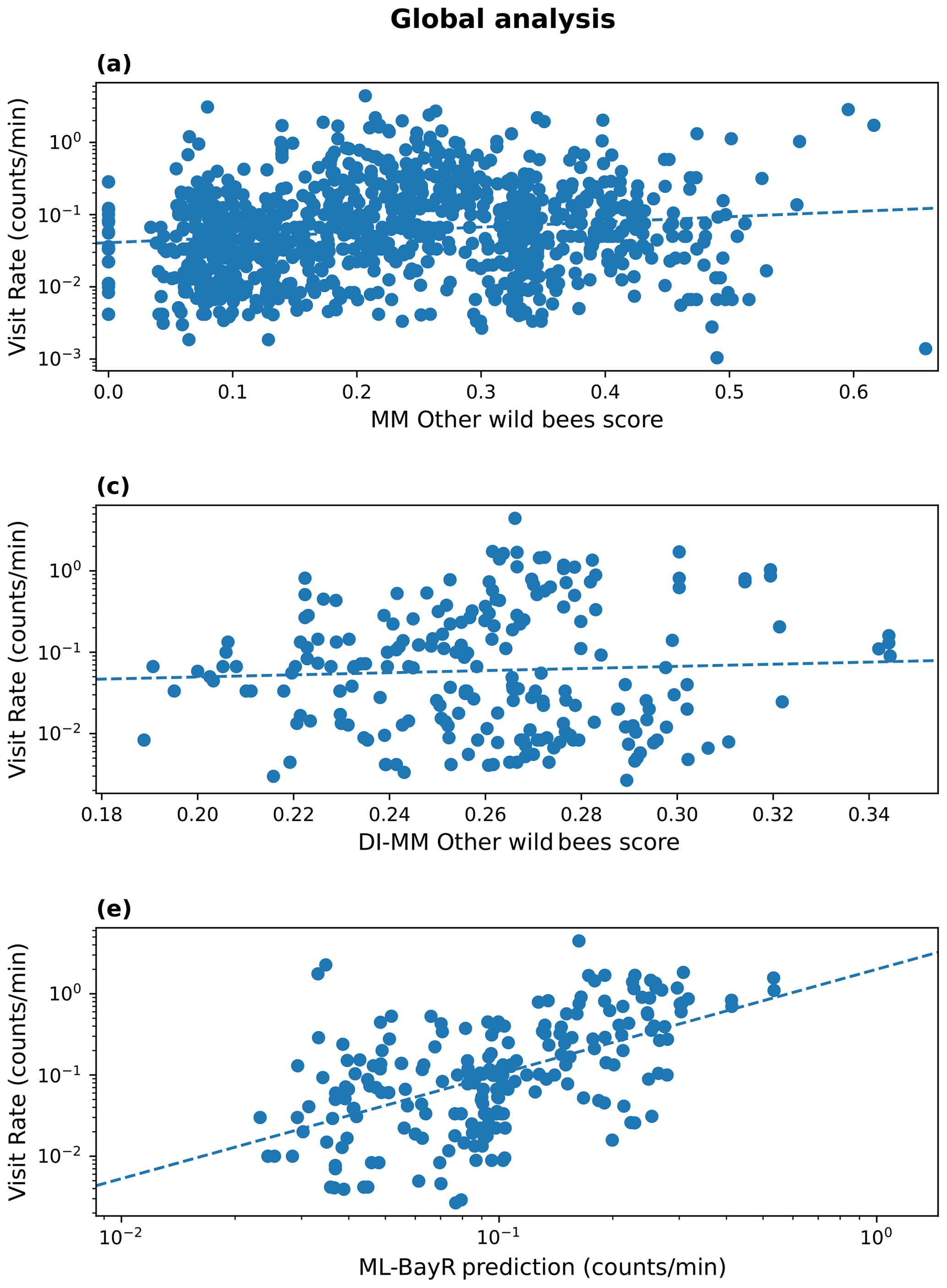
Figure 1 Results at a global scale. Observed visitation rate (counts per minute) versus MM-predicted score (pollinator activity configuration) for other wild bees (a), DI-MM-predicted score for other wild bees (b), and ML predictions of visitation rate (counts per minute) using the Bayesian ridge model for bumblebees and other wild bees combined (c). The dashed lines show a linear fit. The S_ρ value obtained in each case is 0.17 (a), 0.00 (b) and 0.56 (c).

At a global scale, we see different offsets of the observed visitation rate of bumblebees depending on the biome (Fig. H1). We do not see this for other wild bees (Fig. H2). The observations show a lower visitation rate in tropical compared to temperate biomes, which is expected based on bumblebees' known distributions (Hines, 2008). Hence, a meaningful analysis of the global data for bumblebees requires the use of the variable biome as a random effect in a linear mixed model. However, in this work we already perform the analysis per biome, so the analysis would be redundant. Therefore, global results are reported only for other wild bees in the MM and the DI-MM.

3.2 Biome scale

At the biome level, results are highly dependent on the biome where we run the predictions (see Table 2). For simplicity, we discuss here the results only from one MM configuration (pollinator activity) and one ML model (BayR), but similar conclusions arise for other MM configurations and ML models. In Fig. 2, we illustrate the results obtained in the biome with more available sites (temperate broadleaf and mixed forests).

Table 2 Metrics obtained comparing, at every biome, predictions and observations: coefficient of determination (r²), Spearman's coefficient (S_ρ), mean absolute error (MAE) and root-mean-square error (RMSE). For the MMs, we show the results of the pollinator activity MM configuration, and for the ML models, those of the Bayesian ridge regressor. At some biomes, the metrics could not be computed using the ML models due to the absence of the biome in the testing set.

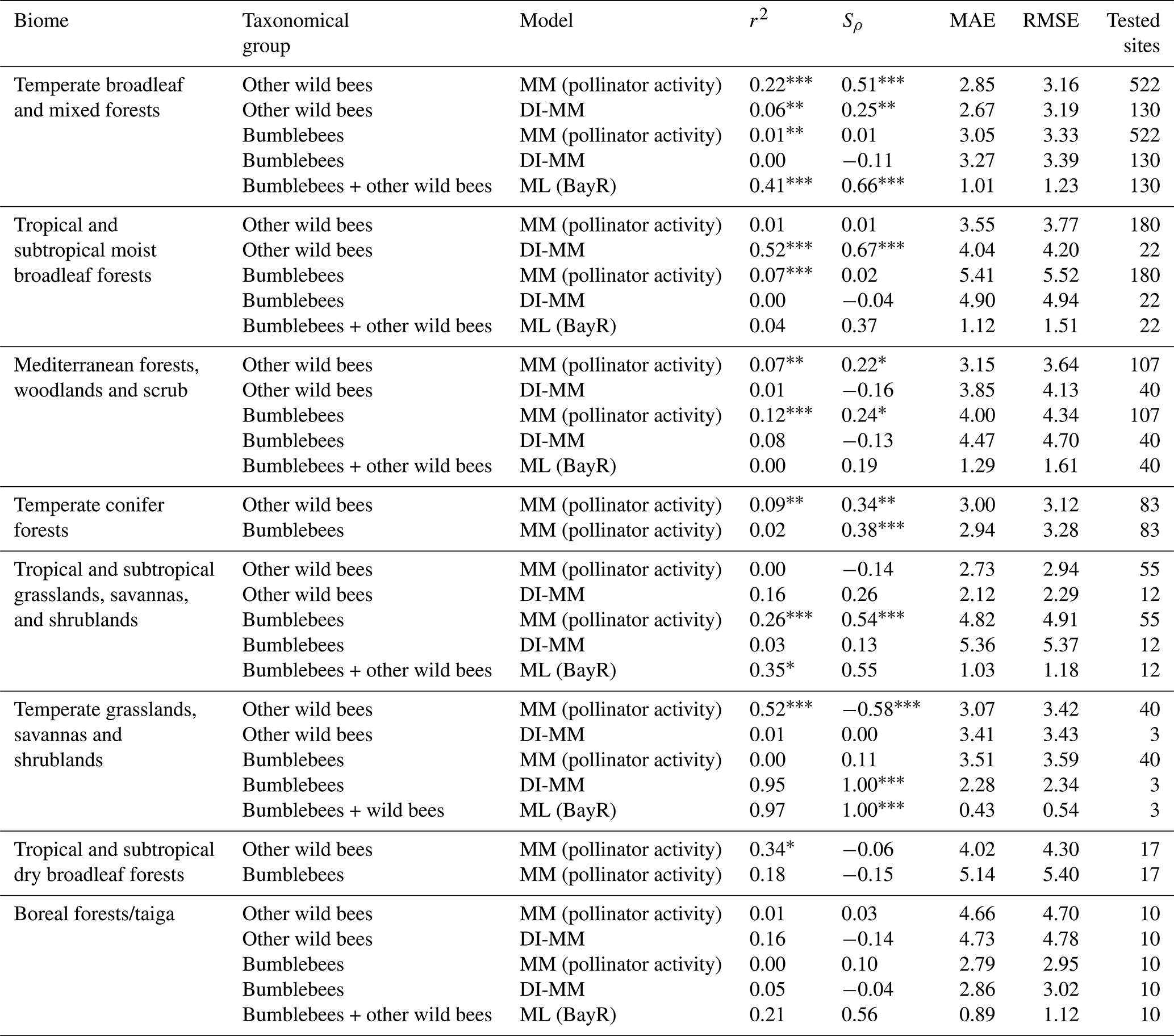
^∗ p value < 0.05. ${}^{\ast \ast }$ p value < 0.01. ${}^{\ast \ast \ast }$ p value < 0.001.

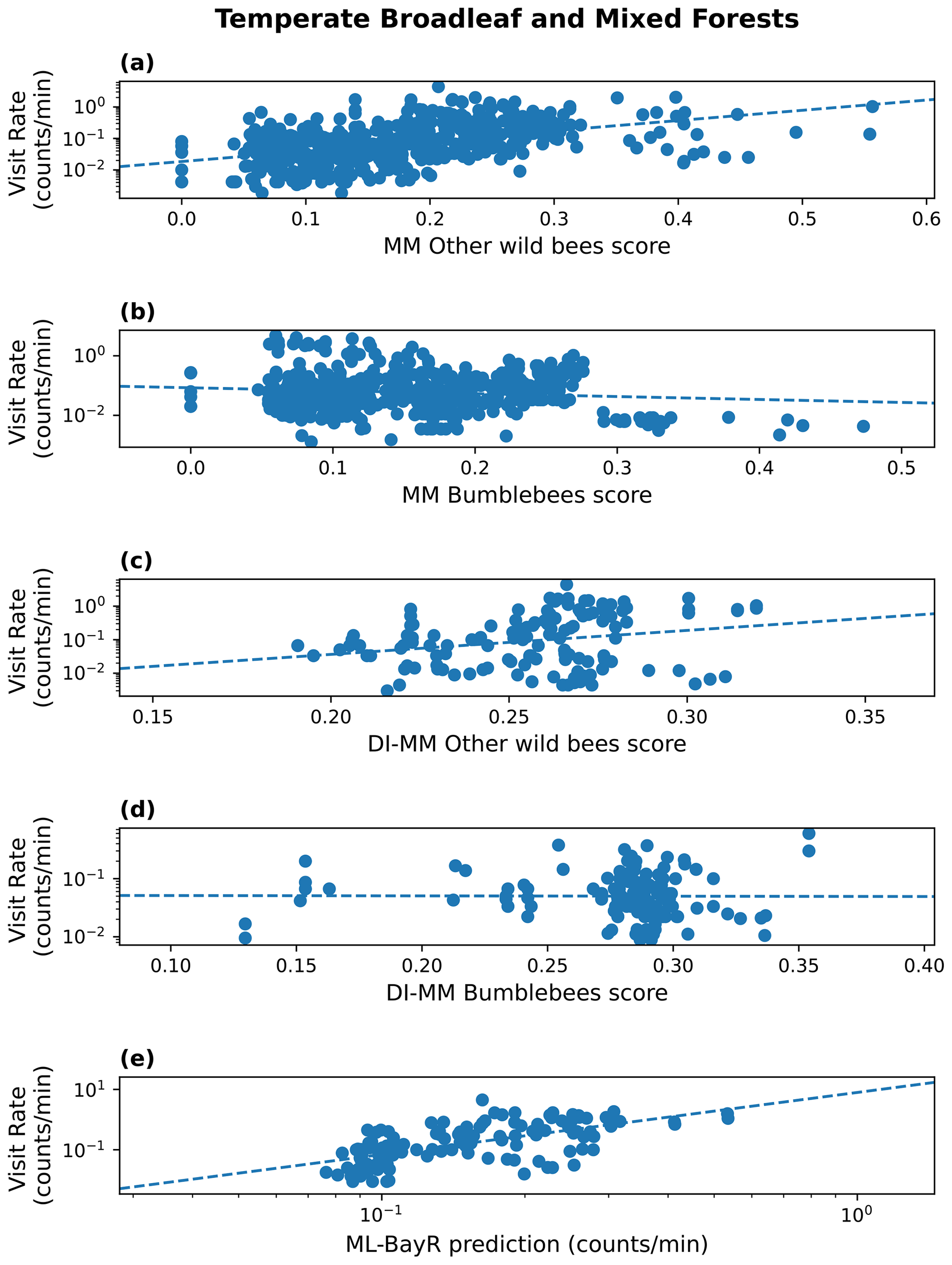
Figure 2 Results in the biome temperate broadleaf and mixed forests. Visitation rate (counts per minute) versus MM score (pollinator activity configuration) for other wild bees (a) and bumblebees (b); DI-MM score for other wild bees (c) and bumblebees (d); and ML predictions of visitation rate (counts per minute) using the Bayesian ridge model for bumblebees and other wild bees combined (e). The dashed lines show a linear fit. The S_ρ value obtained in each case is 0.51 (a), 0.01 (b), 0.25 (c), −0.11 (d) and 0.66 (e).

Considering the group of other wild bees, the MM shows a positive and statistically significant rank correlation in three of the eight biomes: the two biomes characterized by temperate forests (broadleaf and mixed forests (S_ρ=0.51) and coniferous forests (S_ρ=0.34)) and by Mediterranean forests, woodlands and scrub (S_ρ=0.22). The MM performs poorly in tropical biomes, temperate grasslands, savannas and shrublands, and boreal forest. For bumblebees, the MM shows a positive and statistically significant rank correlation in tree biomes: Mediterranean forests, woodlands and scrub (S_ρ=0.24); temperate conifer forests (S_ρ=0.38); and tropical and subtropical grasslands, savannas, and shrublands (S_ρ=0.54).

The use of calibrated tables (DI-MM) does not show good results for bumblebees (only the biome temperate grasslands, savannas and shrublands has a significant rank correlation (S_ρ=1.00) but with only three sites tested), whereas for other wild bees it shows positive and significant rank correlation in two biomes, including the one with the largest number of studies (temperate broadleaf and mixed forests (S_ρ=0.25) and tropical and subtropical moist broadleaf forests (S_ρ=0.61)).

The rank correlation between ML predictions and observations is positive and significant in two of the six biomes present in the test subset: temperate broadleaf and mixed forests, with S_ρ=0.66 (the biome with, by far, the largest number of sites and, thus, the biome that has more impact in the training process), and temperate grasslands, savannas and shrublands, with S_ρ=1.00 (the biome with the smallest number of sites in the test subset, with only three). Moreover, in the other four biomes, the correlation observed was moderate ($S_{\mathit{\rho }}\in [\mathrm{0.19},\mathrm{0.56}]$) but not statistically significant.

3.3 Local scale

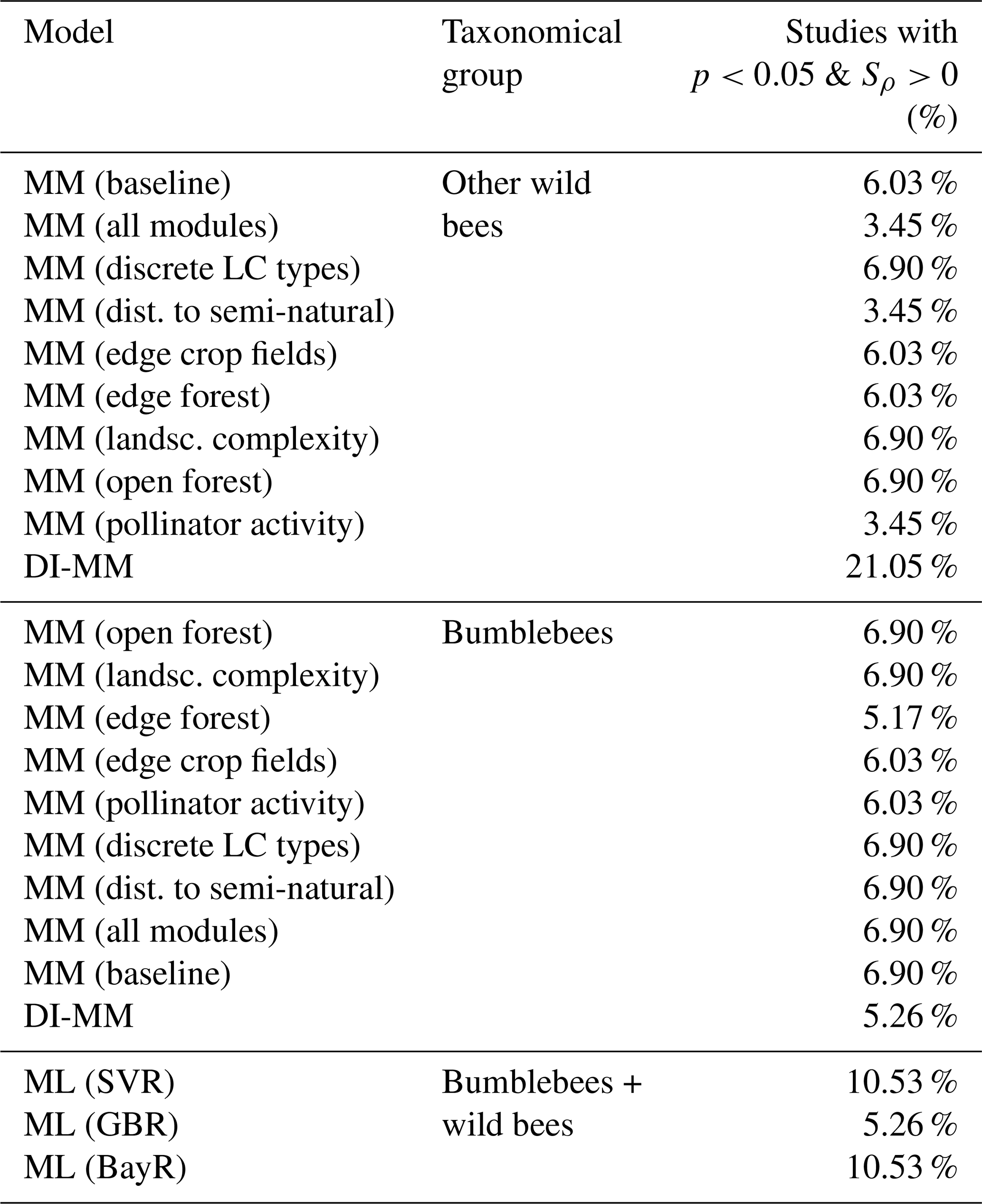
Our results show there is no statistically significant individual rank correlation for most of the studies in CropPol (see Table 3). The model with the largest percentage of studies (21.05 %) showing agreement is the DI-MM for the group of other wild bees.

Table 3 For each model, the percentage of studies where we found a positive and statistically significant rank correlation (S_ρ).

We further explore whether the agreement of the predictions with the observations depends on factors such as the landscape variability, management practices and pollinator dependency of the crop (extracted from Klein et al., 2007), but we do not see any pattern dependent on those factors (Fig. I1).

3.4 Variable importance in ML models

Variable importance for each model is described in Fig. 3. For the BayR model, the most important variables are mean diurnal range, management, elevation and annual mean temperature. The GBR also gives special importance to these four variables, in addition to shrubland cover, soil bulk density and direct evaporation from the soil. The SVR's predictors were all of similar importance. During the exploration process, variables related to the crop cultivated at each study site were taken into account. However, this information was not incorporated into the models as it added complexity without improving the models' fit significantly.

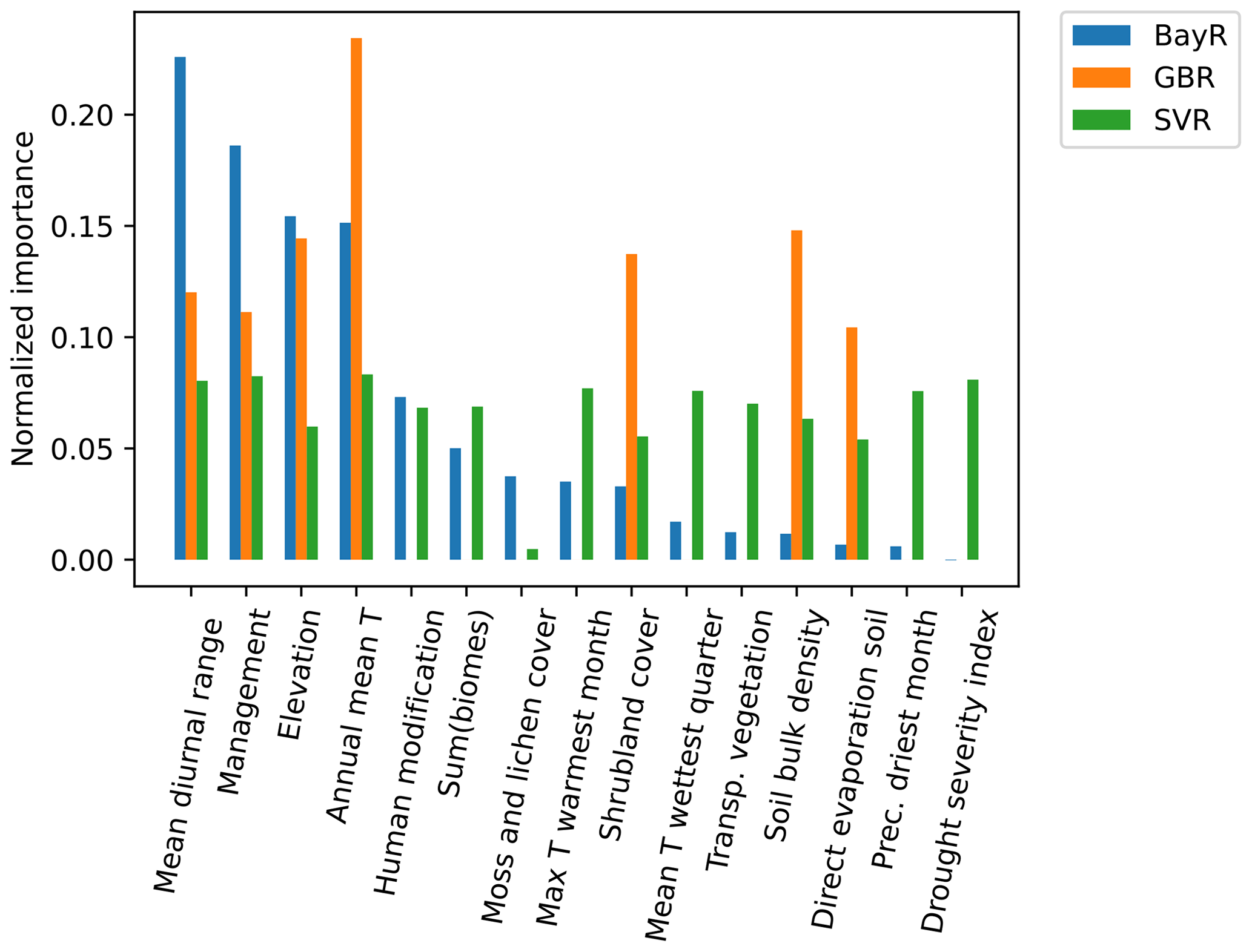
Figure 3 Normalized feature importance computed for three ML models: support vector regressor (SVR), Bayesian ridge (BayR) and gradient boosting regressor (GBR). Feature importance values were normalized in each model so that the sum equals 1. The predictors used for biomes and crops are the result of a one-hot encoding of two formerly categorical features (i.e. one variable is decomposed into several true or false variables). To report their importance in the models, we show the sum of the importance of all these decomposed predictors. Abbreviations (here and later in the text): Transp. vegetation, transpiration from vegetation; Prec. driest month, precipitation of driest month.

3.5 Model selection decision flow chart

Given the results obtained, shown in the previous sections, we show in Fig. 4 a model selection decision flow chart. A hypothetical stakeholder, interested in applying a pollination supply model, can follow the steps described in the flow chart to decide on the most suitable model depending on the study area and data available. Some questions in the flow chart include quantitative indicators to hint at the meaning of the concepts local scale and enough data for ML. We stress that these quantities are just a guide because the exact meaning of these concepts depend on other factors. For example, for the application of an ML model, the dataset must include a variety of patterns that reflects the context of the area where the model is applied. In addition to the number of records, factors like data quality, diversity, representativity and independence must be considered when evaluating the convenience of using ML.

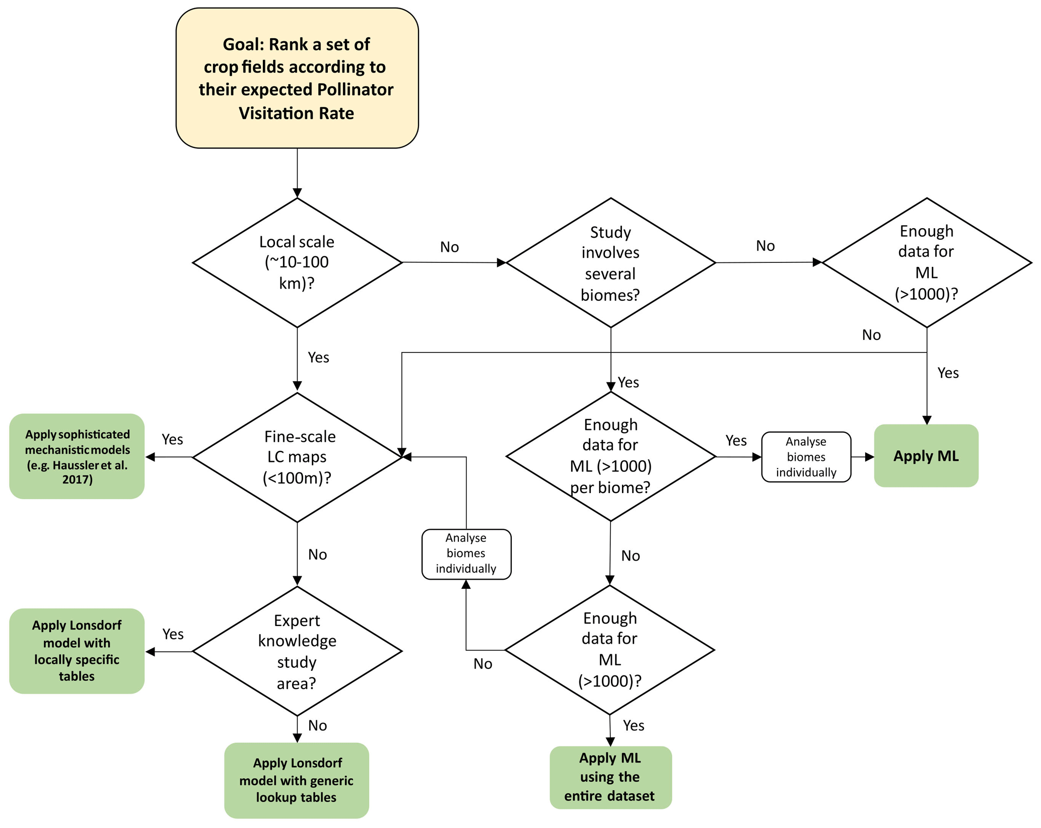
Figure 4 Model selection decision flow chart to show the steps that a stakeholder can take to decide on the most suitable model.

4 Discussion

In this study, we assessed and compared the capacity of a mechanistic model (MM), a data-informed mechanistic model (DI-MM) and machine-learning (ML) models to provide reliable predictions of rates of pollinator visitation to crop fields. The three model types were evaluated in terms of their capacity to rank sites correctly at three geographic scales: local (study by study), individual biomes and global. The MM and DI-MM, which require different inputs depending on the traits considered by the models (in this case foraging range and nesting and floral preferences), were evaluated for bumblebees and other wild bees separately. The ML models, in contrast, were evaluated using the data for bumblebees and other wild bees combined to increase the number of input data, which is critical for data-driven models.

The ML models, in particular the Bayesian ridge regressor, performed well at the global level (S_ρ=0.56). The ML models also worked well at the biomes where more data are available, with S_ρ of up to 0.66. The MM, when applied to the group of other wild bees, gives moderately good results at the global level ($S_{\mathit{\rho }}\in [\mathrm{0.12},\mathrm{0.17}]$) and performed well at the biomes characterized by temperate and Mediterranean forest ($S_{\mathit{\rho }}\in [\mathrm{0.22},\mathrm{0.51}]$). For bumblebees, we observe three biomes with good fits between the MM scores and the observations. Finally, the DI-MM provides good results for the group of other wild bees at the biome with more test sites (S_ρ=0.25). This model also gives, in the group of other wild bees, the highest percentage of studies with a positive and statistically significant rank correlation (21.05 %).

The results obtained at different biomes show that the MM, at least for other wild bees, works best in biomes dominated by temperate or Mediterranean forests. The input table was made from expert opinion by co-authors of this work with no differentiation between biomes, based on global pollinator abundance scores per land cover type (Alejandre et al., 2023). As highlighted by Gardner et al. (2020), expert-based tables can also suffer from different types of bias. In this case, the three biomes where the MM performs well for other wild bees are in Europe or the USA, which are the geographic regions with which the authors of the input table are more familiar. Thus, we cannot rule out the possibility that the expert-based tables used in this work suffer from a significant bias that makes the MM more applicable to geographic regions that are more familiar to the expert contributors.

Even though mechanistic models have previously estimated pollination supply at a continental scale, beyond the extent of biomes (e.g. Zulian et al., 2013), they have not done so globally. Thanks to the data available in recently compiled databases like CropPol, we could prove that it is feasible to use the MM (with relatively simple lookup tables) to compute reliable predictions at large geographic scales. These lookup tables are an attempt to represent the globally averaged preferences of pollinators. However, it is also clear that tables of floral and nesting resources that work well in particular biomes do not necessarily yield good results in other biomes. Indeed, the scores are directly associated with the behaviour of bee species and most species are specific to particular biomes. Looking at the results for bumblebees, the convenience of not applying the MM beyond the extent of biomes seems even stronger. At the global scale, we observe that different biomes show very different visitation rates. Consequently, it would be sensible to use specific lookup tables for each biome if applying the MM to a geographic scale greater than one biome, such as continents. Otherwise, we must use the estimations of the MM with caution.

As an additional modification of the original MM, we used a training set to calibrate the input tables of floral and nesting resources. This approach, i.e. using data instead of expert opinion to inform the input tables of the models, was investigated in detail by Gardner et al. (2020). These authors calibrated the input table of a more sophisticated process-based model using data collected across Great Britain and obtained very good results in terms of r², more so than the moderately good rank correlation obtained here with the DI-MM. The reason for a higher agreement in Gardner et al. (2020) probably arises from the use of a more sophisticated process-based model, a detailed calibration of the tables that included feedback from expert opinion and the application of the models at a much smaller geographic scale (Great Britain versus global). However, looking beyond r², Gardner et al. (2020) warn of the risk of getting unrealistic parameter values from a purely data-driven calibration of the tables. In that regard, the two approaches are complementary: on the one hand, using observational data to inform the input tables of mechanistic or process-based models can potentially overcome the difficulties of computing predictions where expert knowledge is limited; on the other hand, expert knowledge is essential to assess the plausibility of the scores and is the most reliable source of information for those habitats where observational data are scarce.

When analysing the importance of the variables in the ML models, we see that the models use the set of features in different ways (Fig. 3). The SVR is the model that distributes the weight more evenly among the variables, in contrast to the GBR, which mainly uses seven variables. In any case, the three models consider a mix of bioclimatic variables and other variables, such as organic management practices (yes or no), elevation or shrubland cover. Therefore, having a diverse range of variables that adequately describe each location is crucial for achieving a good performance of the ML models.

To our knowledge, this study is the first to globally validate the mechanistic model by Lonsdorf et al. (2009). Moreover, it is also one of the first studies that uses ML models to compute predictions of pollinator crop visitation rates. Kammerer et al. (2021) also used an ML model (a random forest) to predict the pollinator visitation rate, but the methodology that the authors apply prevents us from a direct comparison. The search for parameters is a crucial step in any ML pipeline, and it is key that their test set does not participate in the process. Furthermore, Kammerer et al. (2021) evaluate the model's performance using 10-fold cross-validation on the same dataset used to select the parameters of the ML model. In contrast, we paid particular attention to having a test set completely independent of the training set.

Whenever the extent of the area of interest covers several biomes and the necessary expert knowledge for elaborating specific tables for each biome is not feasible, we have shown that data-driven approaches can be an excellent option to predict pollination supply. The ML models performed well at a global level, with a statistically significant S_ρ of 0.56. The ML models also perform very well in the biome with most available records (temperate broadleaf and mixed forests), with S_ρ=0.66. The DI-MM works moderately well for the group of other wild bees in situations where more data are available, as expected for a data-driven method, i.e. at the biome with the greatest number of sites (S_ρ=0.25).

The global scope of this study gives rise to certain caveats. An important one is that we require data from different studies and regions, collected using different methodologies and at different times of the year. The raw input data are heterogeneous, and this affects the validation process. The methodology used here harmonizes the data, but it also comes at the cost of some data pruning. Moreover, an additional limitation is that the land cover maps used here do not have specific categories for individual crops or at least for pollinator-dependent and non-dependent crops. This is important because pollinator-dependent crops influence wild-bee populations in different ways. Such effects may prove favourable if an adequate number of semi-natural habitats are present in the vicinity, by means of facilitating the provision of food resources (Westphal et al., 2003; Holzschuh et al., 2012). These impacts may be detrimental if the benefits are diluted by an overabundance of this form of land cover type (Holzschuh et al., 2016; Eeraerts et al., 2021). Given that the models have been run on spatial layers available at a global scale, the thematic resolution cannot be as fine as the resolution of other land cover products focused on specific regions or countries. The spatial resolution is also coarser than the one needed to capture the effect of micro-habitat differences. This is a probable cause for the poor results observed at the local scale. Fine-scale land cover inputs also enable the application of more sophisticated MMs (Häussler et al., 2017), thereby augmenting the capabilities of MMs. More sophisticated models can be considered for ML too. In addition to the ML models tested in this work (i.e. the set of models available in the Python library scikit-learn), exploring the use of XGBoost or deep learning models would be very interesting. In summary, there is significant scope to apply more sophisticated MM, DI-MM and ML models, which would allow for more refined performance comparisons.

5 Conclusions

Our study shows the different applicability of model types at different spatial scales, as shown in the model decision flow chart in Fig. 4. For farmers, who might be interested in relatively local interventions, the MM is a good option as long as enough ecological knowledge is available to provide realistic input tables for the MM. However, ML models can fill the gap in those situations where such ecological knowledge is missing. The quality of these models is dependent on the quality of the observational data, but we have shown in this work that currently available open datasets provide the opportunity for them to be run at virtually any place (with many limitations, for example the representativeness of the observational data when applied to a completely different area of study or the spatial and thematic resolution of global datasets). Moreover, there are tools freely available online, such as k.Explorer (IMP, 2023), that facilitate the computation and visualization of pollination service models for users not familiar with coding. Despite the MM being potentially applied over large regions (Image et al., 2022), the ML models seem a very useful approach for policy-makers or landscape managers, who usually need to characterize very wide geographic extents. Regarding the variables present in the ML models, the three models assign different weights. However, they have in common the need to consider a combination of bioclimatic variables and other variables such as management practices, elevation or shrubland cover.

Appendix A: New modules in the mechanistic model

New modules have been added to the original model by Lonsdorf et al. (2009) to test whether they increase the agreement of the model with the observations. The character of these new modules is merely exploratory, and, as such, they are implemented in a simplistic way. The new modules can be classified into two categories according to the type of impact that they are expected to have on pollinators. The first type consists of features that enhance the expected availability of flowers (in terms of quantity or diversity). Therefore, they are used to modify the scores on floral resources, adding a bonus that ranges between 0 and 0.25, depending on the conditions at each location. The range (0–0.25) was set arbitrarily, with the aim of adding a moderate boost to those areas where landscape properties are favourable to pollinators. Given that each module of this type can incrementally increase the floral score of every pixel by 0.25, the combined effect of more than one module can yield very high (and unrealistic) bonus values. To avoid this, we use a bonus value equal to the maximum of them all. In addition, we enforce the condition that the final floral score can never be higher than 1. The following four modules are of this type:

• Forest edges. Floral resources tend to be more abundant at the edge of forests because of the higher availability of light. A bonus of 0.25 is assigned to the pixels at the edge of the forests.

• Forest openness. Similarly to forest borders, light is more accessible in more open forests or forest patches. We use the inverse of the tree canopy cover and scale the values to the range between 0 and 0.25, and we assign that bonus to forest pixels.

• Crop field size. Reducing the size of the fields has a positive effect on pollinators (Fahrig et al., 2015). We included this effect indirectly, by means of identifying the borders in crop fields (defining crop field as connected area classified as annual crop). For the same total area, the length of the field borders will be larger when the fields are smaller. The floral score of those pixels identified as crop field border is incrementally increased by 0.25.

• Landscape complexity. The MM factors in the effect of the surroundings by the fact of using the flight distance, but it actually does not capture the landscape complexity, in the sense of having different land cover types in the crop field surroundings. We modelled this effect by computing the number of different land cover types (neglecting water and urban types), within a radius equal to the typical distance of flight. We set a cut-off value of 5, meaning five or more land cover types within the considered radius meant a maximum bonus of 0.25.

The second type of additional module covers those features that do not change the landscape suitability but modify the expected visitation rate. This is modelled applying a factor to the MM score that aims to model the decay of the visitation rate under certain conditions. We applied two of these modules.

• Pollinator activity. The activity of pollinators strongly depends on the temperature of their bodies, which in turns depends directly on the ambient temperature and solar irradiance (Corbet et al., 1993). A similar component has been applied in the past by other authors as a component of mechanistic models (Zulian et al., 2013; European Commission Joint Research Centre, 2018). It is based on a linear relationship, found by Corbet et al. (1993), between the temperature and the percentage of active insects, using the black globe temperature as an approximation for the temperature of the insect bodies. The pollinator activity (A_pollinator) is computed as follows:

  $$\begin{array}{}\text{(A1)}& {\displaystyle }\begin{array}{rl}& T_{\mathrm{bg}}^M=\\ & \left\{\begin{array}{ll}\mathrm{0}& \text{if }{T}^M<T_{min},\\ -\mathrm{0.62}+\mathrm{1.027}{T}^M+\mathrm{0.006}{R}^M\frac{\mathrm{24}}{d}& \text{otherwise,}\end{array}\right.\end{array}\text{(A2)}& {\displaystyle }{T}_{\mathrm{bg}}=\underset{M}{max}\left\{T_{\mathrm{bg}}^M\right\},\text{(A3)}& {\displaystyle }{A}_{\mathrm{pollinator}}=f_{\mathrm{0}}+f_{\mathrm{1}}{T}_{\mathrm{bg}},\end{array}$$

  where $T_{\mathrm{bg}}^M$ is the black globe temperature for month M in degrees Celsius, T^M is the average temperature of air at 2 m above the surface for month M in degrees Celsius (using ERA5-Land monthly averaged data; Muñoz Sabater, 2019) and R^M is the average solar radiation in W m⁻² for month M (using TerraClimate; Abatzoglou et al., 2018). The variable d stands for day length in hours, is computed using the equations in Forsythe et al. (1995) and is used to obtain average solar radiation during the day from R^M. The parameters T_min, f₀ and f₁ depend on the taxonomical group. Corbet et al. (1993) find coefficients for honeybees and bumblebees. We used the parameters of honeybees for our group of other wild bees given that the size of honeybees is more comparable to the typical size of the individuals in this group. T_min stands for the minimum air temperature for pollinator activity, while f₀ and f₁ are the regression coefficients obtained by Corbet et al. (1993). The maximum value of $T_{\mathrm{bg}}^M$ is used because we assume that measurements are normally taken in periods of high pollination activity. In the case A_pollinator>1, the value is capped at 1.

• Distance to semi-natural land. Pollination supply is sensitive to the distance to semi-natural areas, as shown in Garibaldi et al. (2011). Even though the model already takes this into account implicitly (by giving higher scores to land cover types classified as semi-natural and weighting them by the distance to the computed pixel), European Commission Joint Research Centre (2018) included it as an additional component of the model to reinforce its importance. In our study, it is included to test whether this reinforcement is relevant or redundant. This module consists of applying a factor, dependent on the distance to semi-natural areas, to the pollinator score S_pollinator. We used the decay rate of the visitation rate from Ricketts et al. (2008):

  $$\begin{array}{}\text{(A4)}& S_{\mathrm{pollinator}}^{\mathrm{modified}}=S_{\mathrm{pollinator}}\cdot e^{-\mathrm{0.00104}\times D},\end{array}$$

  where D is distance to semi-natural areas in metres.

Appendix B: More details on the input data of the machine-learning models

The proportion of each land cover type is computed using a weighted average of land cover proportion with a Gaussian kernel function around each survey site location, with a sigma value corresponding to the typical distance of flight of the taxonomical group. Therefore, one value per taxonomical group is computed. To get a single value, the average was applied. The same procedure (one value per taxonomical group averaged to get a single value) was applied for the variable pollinator activity.

Some variables were extracted from dynamic datasets that are composed of a number of temporal slices (e.g. TerraClimate consists of monthly data). In those cases, we extracted the value of the predictors as the mean using only the date range corresponding to the sampling year of the associated site in CropPol. In cases where the sampling year was out of the temporal boundaries of the dataset, we averaged over the whole temporal range of the dataset.

We analysed the collinearity of the numeric predictors and clustered them hierarchically. With that aim, we first computed the Spearman correlation matrix M_ρ and defined a distance matrix ${\mathbf{M}}_{\mathrm{D}}=\mathrm{1}-{\mathbf{M}}_{\mathit{\rho }}$. Then, we performed Ward's linkage on that matrix to aggregate predictors hierarchically (see Fig. F1). The clusters of predictors finally selected depend on a threshold of the distance between them. To set such a threshold, we performed cross-validation in the training set within an interval of values, and we selected a value for the distance of 0.75 in order to have the maximum level of clustering while keeping the mean Spearman's coefficient high (see Fig. F2). With that threshold, we obtained 13 clusters from the original 56 numeric predictors, as shown in Table F2. In addition, we checked the variance inflation factor of the variables, and the maximum value was 9.22, below the critical threshold of < 10 proposed by Dormann et al. (2012) as a rule of thumb.

The categorical variables terrestrial biome and crop species were transformed into numerical values by one-hot encoding; that is to say, each category of those variables is used to create a new predictor with only two possible values: present (1) or not present (0). The variable farming management practices was transformed into numerical values from 0 to 3 by ordinal encoding, with the management options ordered according to pollinator friendliness: conventional (0), integrated pest management (1), unmanaged (2) and organic (3). Sites where management practices were unknown were assumed to be conventional. After these transformations, we had a total number of 97 numerical predictors (Table F1). As mentioned above, the collinearity analysis enabled the clustering of 56 predictors into 13 clusters. Moreover, four crops and one biome were not present in the training set, and the corresponding variables created by one-hot encoding could be removed from the training set. Therefore, we removed 48 predictors from the total number of 97, and used a final number of 49 (1 variable for management, 8 for biomes, 27 for crops and the already-mentioned 13 numeric representing the 13 clusters of 56 predictors)

Appendix C: Filters

The records present in CropPol (3394 sites) were filtered to ensure that enough information was available for the analyses and that the input data for these analyses were as coherent as possible (e.g. harmonizing units of the pollinator visitation rate). We prepared three datasets:

• Dataset-1 (1403 records), for the analyses using the MM at the local scale;

• Dataset-2 (1027 records), for the analyses using the MM at the scales of biomes and global, where the abundances must be harmonized across different studies;

• Dataset-3 (1007 records), for the analyses involving the split of the data into training and test subsets.

We applied six common filters to the preparation of the three datasets and then particular filters for each of them. After applying the common filters, the filtered dataset contains 1416 records (42 %). These common filters are as follows:

1. Coordinates defined (3022 records). The coordinates refer to the position of each field sampled in the study.

2. At least one taxonomical group with abundance higher than 0 (1926 records). Absences were not considered because two records with 0 abundance cannot be harmonized with respect to sampled time; i.e. two absences would be equal regardless of whether they were observed during 1 min or 1 h.

3. Observations more recent than 1991 (3377 records). This filter ensures that the temporal boundaries of the input datasets are not far from those years. After the application of the filters, the oldest observation dates from 2001.

4. Sampling method different than pan trap (2226 records). Pan traps attract insects and, as such, increase the number of observations in relation to other methods (Portman et al., 2020).

5. Integer values at every site, with a tolerance of 0.05 (3309 records). This filter is meant to harmonize, to some extent, the methodology used by the contributors to CropPol, in terms of how the abundances are reported. The tolerance is set because some authors in CropPol add a small amount (e.g. 0.01) to the abundance value as a flag for rare specimens, but it does not have any effect on the integer part of the actual abundance value. On the other hand, some authors report abundances in different units, e.g. observations per flower per minute, that were processed by the data curators of CropPol in order to register total abundance values in the same units (number of observations). We preferred to use the studies that report number of observations directly. In any case, this filter removes only a few records from the dataset (85 records, only 0.25 % of the total number).

6. Coordinates vary within the study (3366 records). The goal of this filter is to rule out sites with inaccurate coordinates because it is not possible that every site has the same coordinates if their positions are accurately defined in the dataset.

After the application of the common filters, the additional filter to obtain Dataset-1 is as follows:

• Studies with at least three sites (1403 records, 116 studies). Harmonization of measurements using the total sampled time was not needed because sampling effort was consistent across sites within every study.

After the application of the common filters, the additional filter to obtain Dataset-2 is as follows:

• Defined sampled time (1027 records). We harmonize measurements across studies using the total sampled time (see Sect. 2.2). Hence, we must have a value for this variable in every site of Dataset-2. This filter was not necessary for the analysis at the local scale because sampling effort was consistent across sites within studies.

After the application of the common filters, the additional filters to obtain Dataset-3 are as follows:

• Defined sampled time (1027 records).

• Fewer than seven not defined values of environmental variables per site (1389 sites). The value of many environmental variables at the coordinates of a few sites is not defined due to a lack of coverage of the input datasets at these particular locations. We filtered out those records.

Appendix D: The crop pollination database (CropPol)

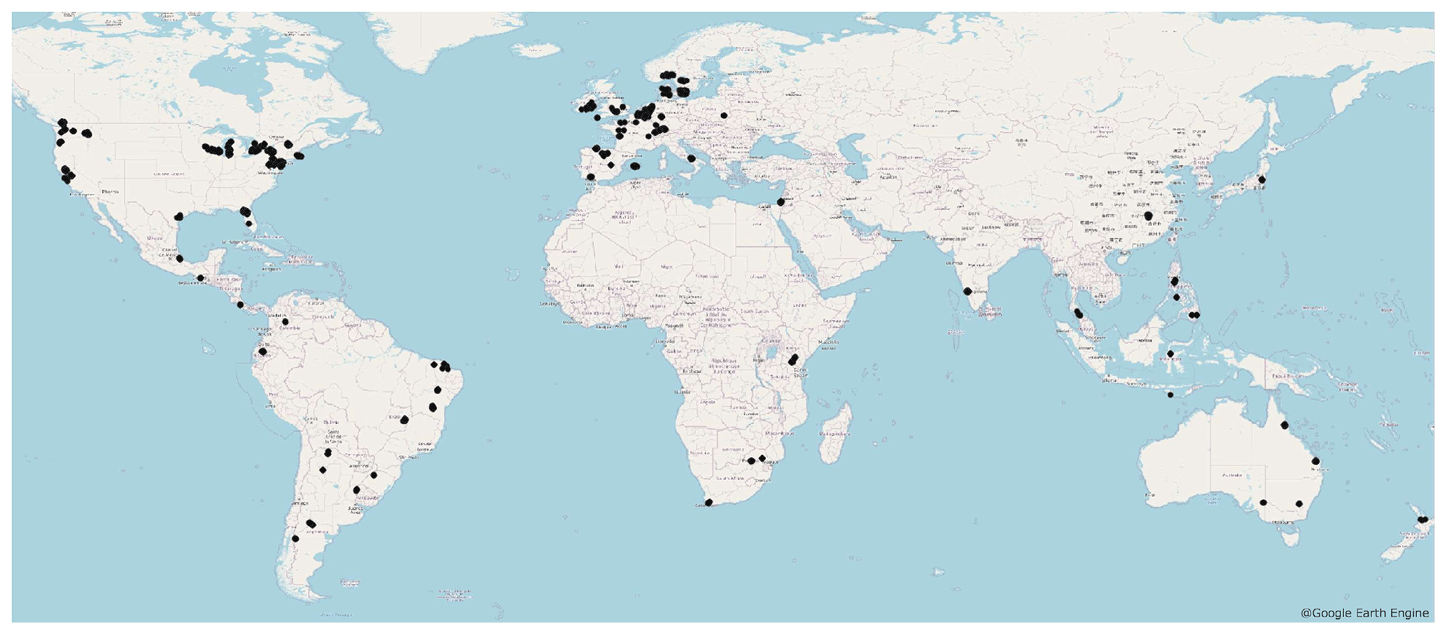
Figure D1 Location of the records available in CropPol. Image generated with © Google Earth Engine.

Appendix E: Input data of the mechanistic models

Table E1 Floral and nesting resource scores (from 0 to 1), when using the land cover map with continuous fields. The floral resource score represents a relative measurement of typical foraging resources when comparing land cover types. The nesting resource score represents a relative measurement of habitat extent suitable for nesting. Values are adapted from the global assessment by Alejandre et al. (2023). Management+ stands for the additional score added to land cover types when evaluating the model in a location where organic farming is practised.

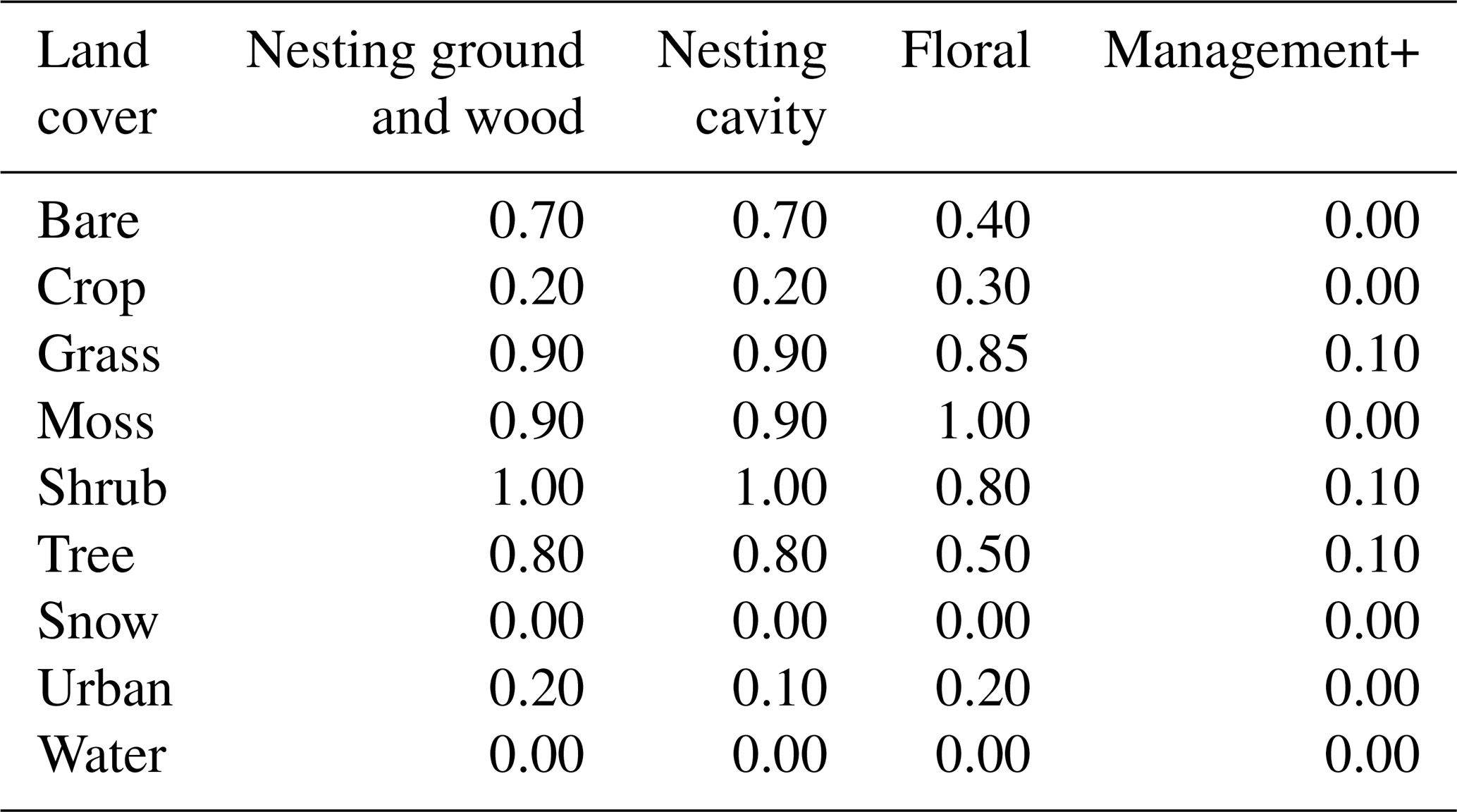
Table E2 Floral and nesting resource scores (from 0 to 1), when using the land cover map with discrete land cover types. The floral resource score represents a relative measurement of typical foraging resources when comparing land cover types. The nesting resource score represents a relative measurement of habitat extent suitable for nesting. Values are derived from the adaptation of the tables used by (Zulian et al., 2013) to the land cover types used in our study. Management+ stands for the additional score added to land cover types when evaluating the model in a location where organic farming is practised.

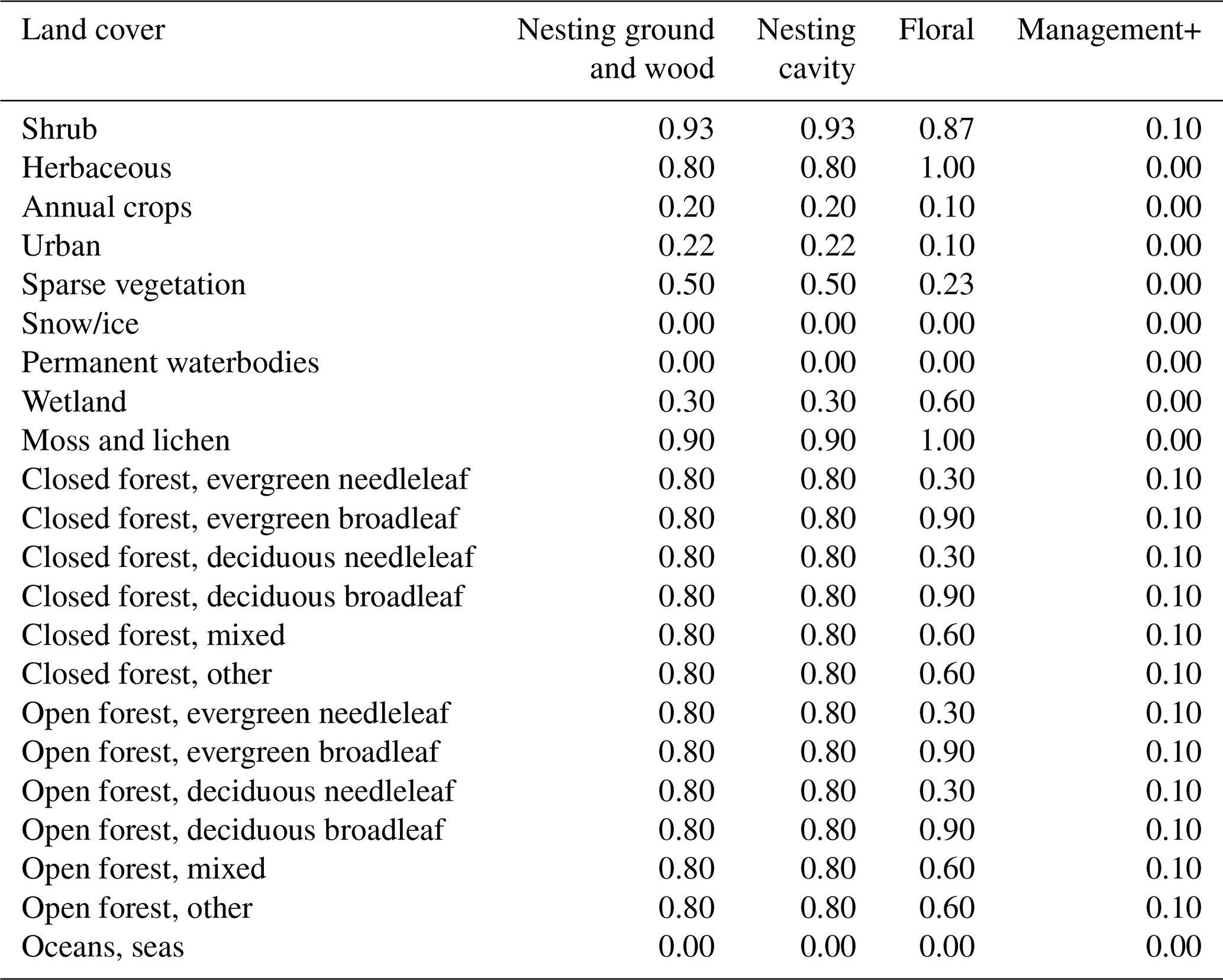
Table E3 Floral and nesting resource scores, obtained for the two pollinator groups (bumblebees and other wild bees), after a calibration process. The floral resource score represents a relative measurement of typical foraging resources when comparing land cover types. The nesting resource score represents a relative measurement of habitat extent suitable for nesting. Management+ stands for the additional score added to land cover types when evaluating the model in a location where organic farming is practised.

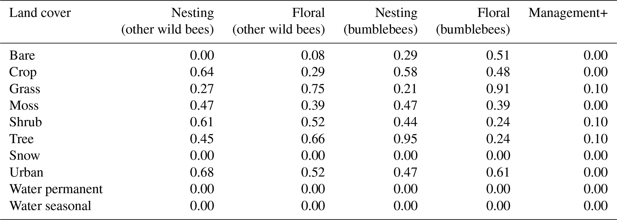
Table E4 Taxonomical groups considered in this work. Distances based on the intertegular span registered in Traitbase (Kendall et al., 2019; Traitbase, 2023) and the parameters found by Greenleaf et al. (2007). Ground nesting refers to nests excavated by the pollinators on the ground. Cavity nesting refers to existing cavities, e.g. burrows and nests of small animals. Other wild bees are mainly soil nesters (Danforth et al., 2019), while bumblebees usually prefer what is defined here as cavities (O'Connor, 2013).

Appendix F: Predictors in the machine-learning model

Buchhorn et al. (2020)Dinerstein et al. (2017)Hengl (2018a)Hengl (2018b)Hengl (2018d)Hengl and Wheeler (2018)Hengl and Gupta (2019)Hengl (2018c)Hijmans et al. (2005)Theobald et al. (2015)Theobald et al. (2015)Jarvis et al. (2008)Running et al. (2017)Zhang et al. (2019)Gan et al. (2018)Zhang et al. (2016)Abatzoglou et al. (2018)Muñoz Sabater (2019)Kennedy et al. (2019)Allen-Perkins et al. (2022)

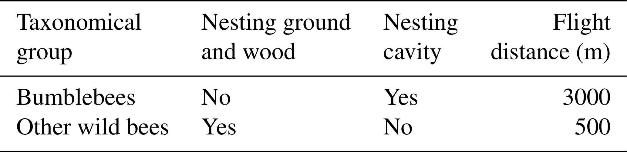
Table F1 Variables used as predictors in the machine-learning pipeline. We also show the dataset from where the measurements were extracted, with a reference.

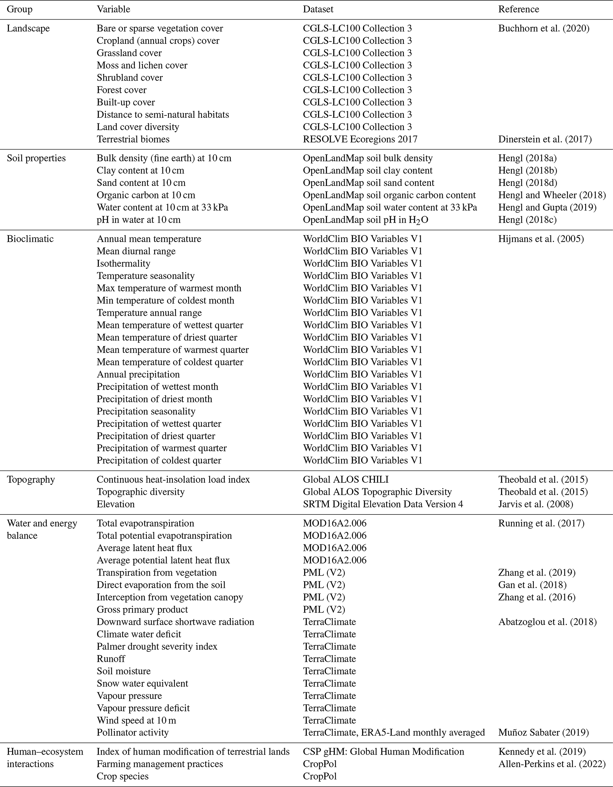
Table F2 Clusters of features represented by the selected features that are used as proxies for the rest of the variables in the cluster. Abbreviations: cont., continuous; evapotr., evapotranspiration; pot., potential; prec., precipitation; dist., distance.

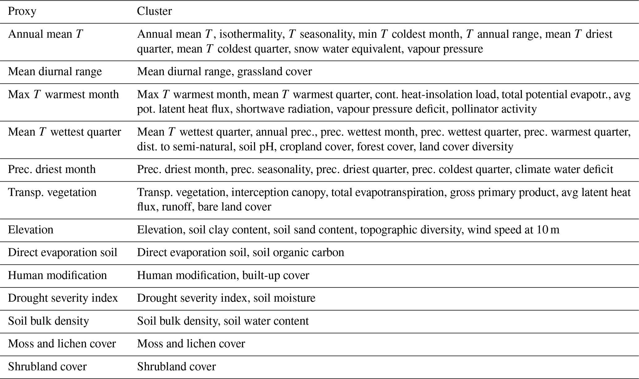
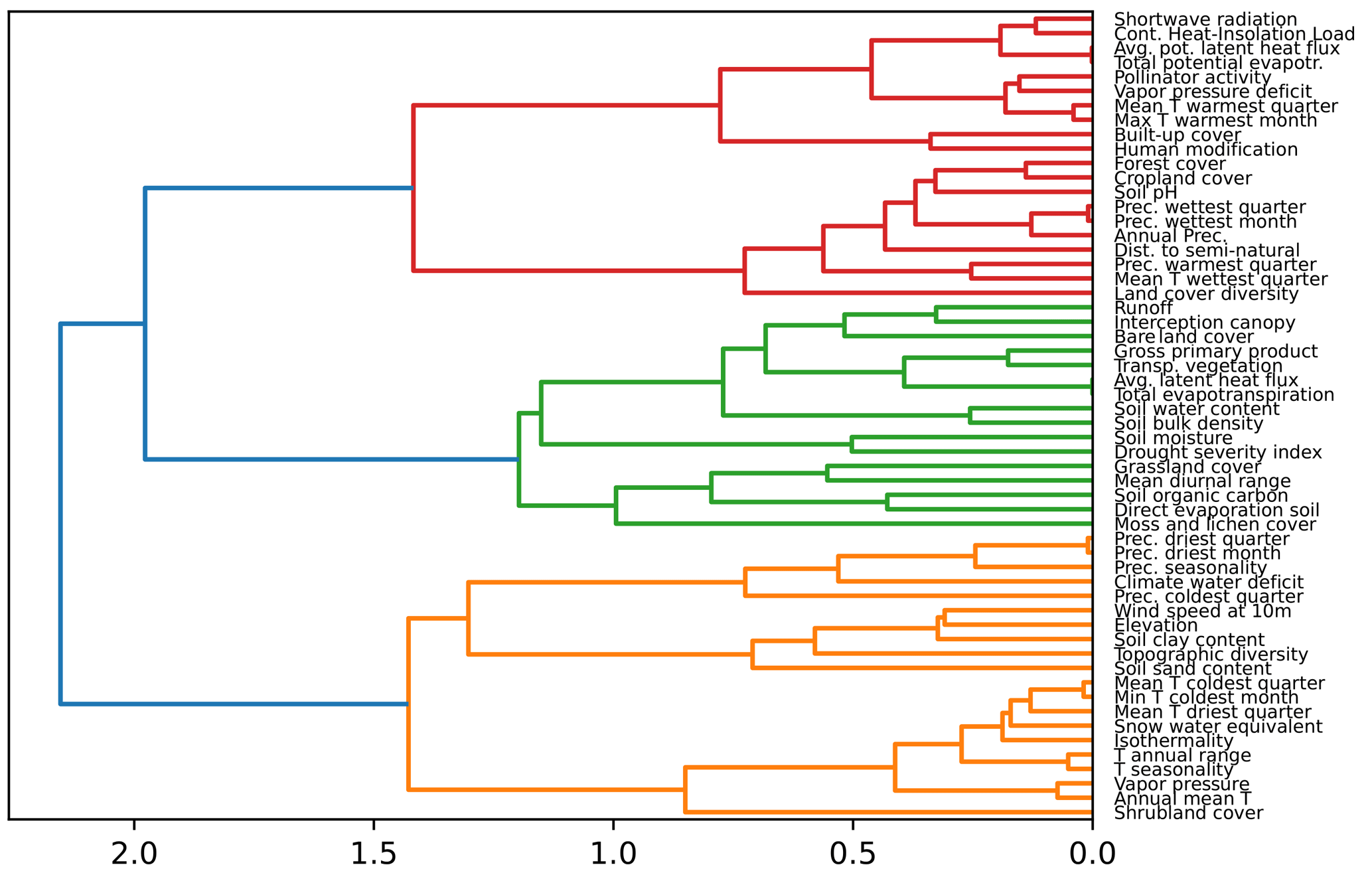
Figure F1 Dendrogram showing the hierarchical clustering of the variables. On the x axis, we show the distance between variables, based on the rank correlation found between the variables and Ward's linkage to aggregate predictors hierarchically. Clusters of predictors can be created selecting a threshold for the distance.

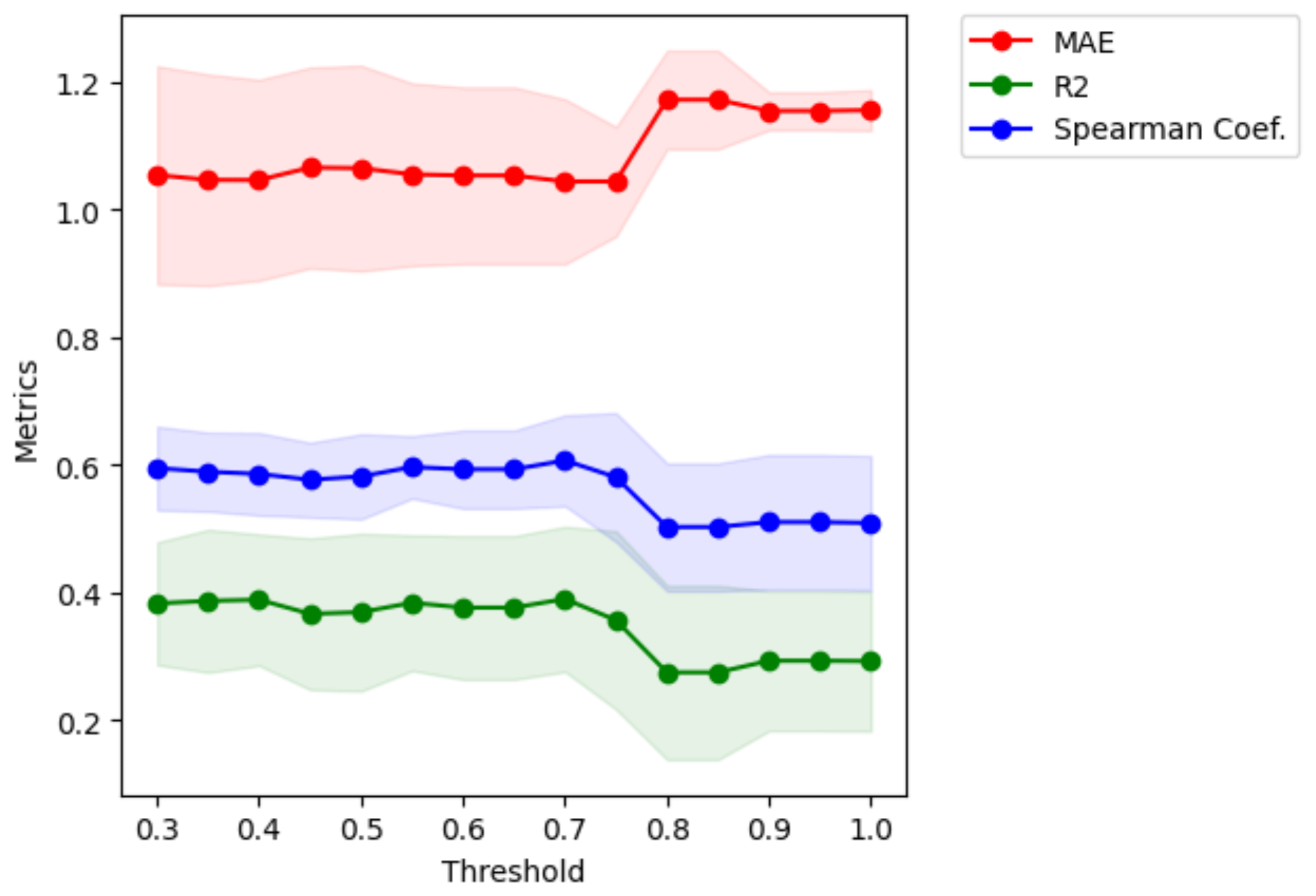
Figure F2 Metrics versus threshold used in the distance to create clusters of variables. Given a threshold value, we obtain clusters of variables that are used to perform cross-validation and compute the metrics MAE, r² and S_ρ. The optimum threshold is the maximum value that keeps the MAE as low as possible and the correlation coefficients as high as possible. In this case, a value of 0.75 was selected.

Appendix G: Biomes

Table G1 Biomes present in this work.

Appendix H: Results at the global scale

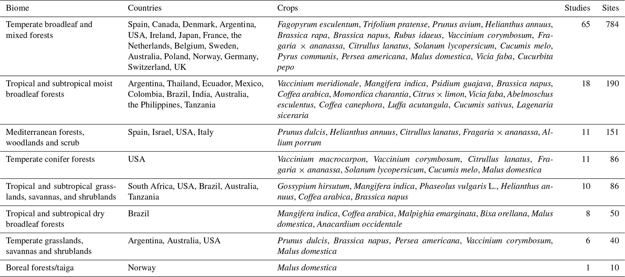
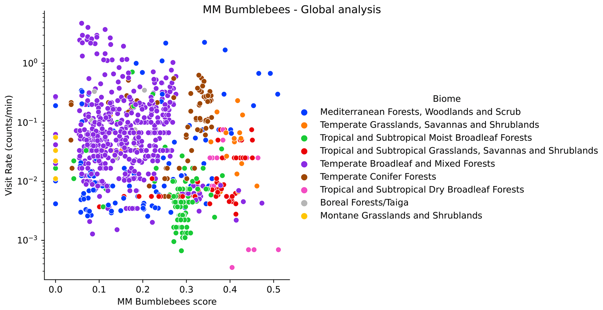
Figure H1 Visitation rate (counts per minute) versus MM scores for bumblebees (using the configuration pollinator activity), at the global scale. We highlight different biomes with colours.

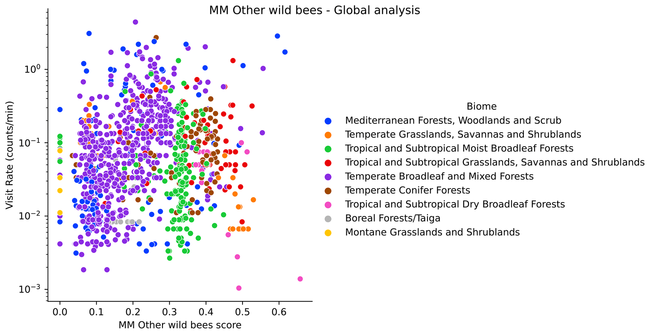
Figure H2 Visitation rate (counts per minute) versus MM scores for other wild bees (using the configuration pollinator activity), at the global scale. We highlight different biomes with colours.

Appendix I: Results at the local scale

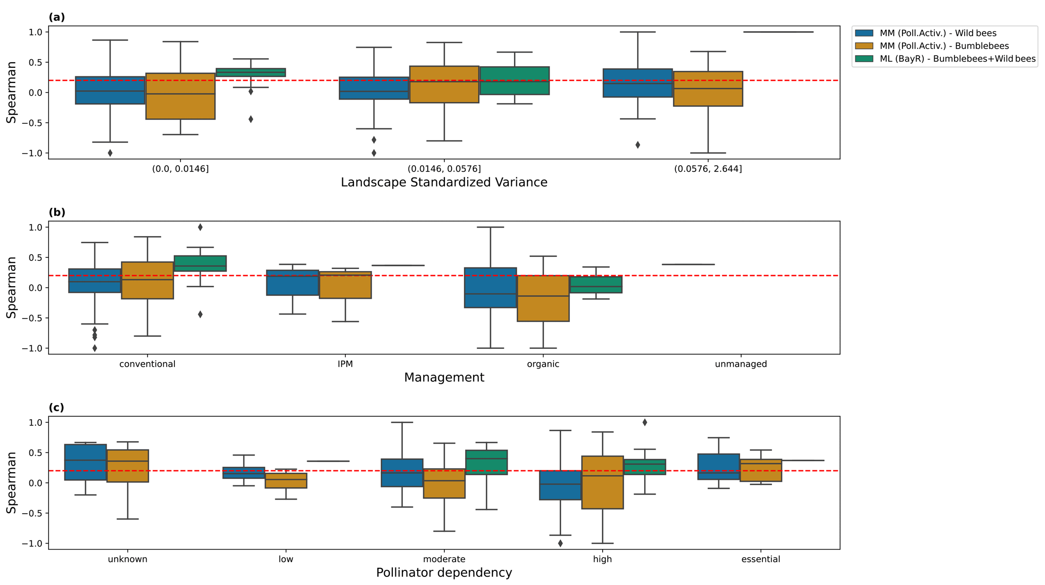
Figure I1 Spearman coefficient obtained comparing, for every study individually, predictions and observations, for the pollinator activity MM configuration (bumblebees and other wild bees) and the ML regressor Bayesian ridge (BayR). We show the results for different levels of the following: (a) landscape standardized variance, computed as the variance divided by the squared mean of the MM scores; (b) farm management practices; and (c) pollinator dependency. The dashed red line, at S_ρ=0.2, is set as an arbitrary threshold for moderate agreement between model and observations. Bin thresholds for landscape standardized variance have been set to values that yield the same number of studies in every bin (taking the MM dataset as the reference because the dataset used for the evaluation of the ML models only includes the studies present in the test set). IPM denotes integrated pest management.