Comment on “Pollination supply models from a local to global scale”: convolutional neural networks can improve pollination supply models at a global scale

Tools to predict pollinator activity at regional scales generally rely on land cover maps, combined with human-inferred mechanistic rules and/or expert knowledge. Recently, Giménez-García et al. (2023) showed that, using large pollinator datasets, different environmental variables, and machine learning models, those predictions can be enhanced but at the cost of losing model interpretability. Here, we complement this work by exploring the potential of using advanced machine learning techniques to directly infer wild-bee visitation rates across different biomes only from land cover maps and available pollinator data while maintaining a mechanistic interpretation. In particular, we assess the ability of convolutional neural networks (CNNs), which are deep learning models, to infer mechanistic rules able to predict pollinator habitat use. At a global scale, our CNNs achieved a rank correlation coefficient of 0.44 between predictions and observations of pollinator visitation rates, doubling that of the previous human-inferred mechanistic models presented in Giménez-García et al. (2023) (0.17). Most interestingly, we show that the predictions depend on both landscape composition and configuration variables, with prediction rules being more complex than those of traditional mechanistic processes. We also demonstrate how CNNs can improve the predictions of our previous data-driven models that did not use land cover maps by creating a new model that combined the predictions of our CNN with those of our best regression model based on environmental variables, a Bayesian ridge regressor. This new ensemble model improved the overall rank correlation from 0.56 to 0.64.

1 Introduction

Spatial modeling of pollinator populations is an effective way to describe the effects of future land-use changes on pollinator availability, identify areas at risk of pollination deficits, and convey this knowledge to stakeholders (Gardner et al., 2020; Polce et al., 2013). Such knowledge transmission is essential to effectively use managed pollinators as well as to support populations of wild pollinators within modern agricultural landscapes. Previous research assessing the fit of different modeling techniques to rank sites by their values of pollinator visitation rates to crop fields (Giménez-García et al., 2023) showed that, overall, the mechanism-free machine learning models tested were more accurate than a widely used mechanistic model (Lonsdorf et al., 2009) and its adaptations, at both biome and global scales. This disparity likely arises from the simplicity of the mechanistic models tested, which are based on assigning separate nesting and flowering quality scores to each habitat for different taxa in land cover maps while accounting for flight distances. Indeed, more sophisticated mechanistic models can yield better results, at least at intermediate scales between individual biomes and global assessments (Gardner et al., 2020). However, they require extensive ecological knowledge, making calibration difficult with noisy, biased, and limited data (Gardner et al., 2020).

In this technical note, we explore the use of deep learning to infer predictive mechanistic rules without explicitly enforcing specific mechanisms, aiming to estimate pollination services using land cover maps on a global scale. This approach could enhance predictive power without losing a mechanistic interpretation and hence help us understand how habitat quality and landscape composition affect wild-pollinator availability. These predictions would be particularly important within areas where expert knowledge is limited and hence it is not possible to calibrate mechanistic models (Giménez-García et al., 2023; Gardner et al., 2020). Unlike classical machine learning, deep learning does not require the prior identification of important data features using expert knowledge (Guyon et al., 2008), which is beneficial when features are not obvious or are difficult to extract, as in image-based maps (Borowiec et al., 2022). Our hypotheses are (1) deep learning algorithms can use image-based maps to extract novel mechanistic rules linking land cover composition and configuration to the pollination services of wild bees, (2) a model based on land cover maps with more complex rules will outperform the mechanistic models previously tested in Giménez-García et al. (2023), and (3) combining predictions from the land-cover-map-based model with other machine learning models using a broader set of environmental variables from Giménez-García et al. (2023) will enhance the overall predictive power.

To test these hypotheses, we used the same subset of visitation rates and site records from CropPol (Allen‐Perkins et al., 2022), a global dataset featuring data on visitation rates to different crops, as in Giménez-García et al. (2023) to create the training and test partitions for our models. The same split for cross-validation was also used to ensure coherence with the results in Giménez-García et al. (2023). We fitted a convolutional neural network (CNN) (LeCun et al., 2010; He et al., 2016), a deep learning model that is particularly well suited for processing image data (see Guyon et al., 2008, for an introduction to the algorithm and Fig. 1 along with Appendix A for our model details). The algorithm was fed with the nine “fraction maps” (19 × 19 pixels, each a 100 m pixel) extracted from the Copernicus Dynamic Land Cover product (Buchhorn et al., 2020) for each location in the training and test datasets (see Fig. A1 for an example). After fitting the CNN algorithm, we adapted the Gradient-weighted Class Activation Mapping (grad-CAM) technique (Selvaraju et al., 2019) to our regressor CNN to identify which parts of the image the CNN focuses on when predicting wild-bee visitation rates. This provided pixel importance estimates for the test dataset maps (Appendix B). To have a glimpse of the rules or mechanisms the CNN algorithm has learned, we used a general linear mixed model (GLMM) to relate pixel importance in the land cover maps to their composition and configuration (Appendix C). Finally, we combined the predictions from the CNN model with those from the best model identified by Giménez-García et al. (2023), the Bayesian ridge regressor (see Guyon et al., 2008, for an introduction to the algorithm and model details in Fig. 2 and Appendix D), by fitting both into a neural network, another deep learning model (Goodfellow et al., 2016). To evaluate their performance, we used the validation procedure outlined by Giménez-García et al. (2023).

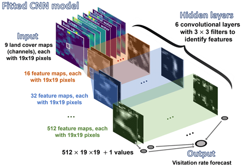
Figure 1 Schematic representation of our CNN model. The algorithm is fed with inputs (tensors) that contain nine layers, each with 19 × 19 pixels. Each layer corresponds to one of the nine fraction maps, providing proportional estimates (i.e., the percentage of a 100 m pixel covered by a specific class of land cover) for vegetation and ground cover types (see Fig. A1 for further details and an example). These layers are extracted from the Dynamic Land Cover product by Copernicus, which provides annual global land cover maps and cover fraction layers for the reference years 2015 to 2019 (Buchhorn et al., 2020).

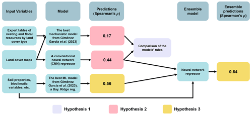
Figure 2 Schematic representation of the relationships between input variables, models, predictions, and ensemble components for predicting wild-bee visitation rates. Arrows indicate connections, with elements used to test the hypotheses highlighted in purple (Hypothesis 1), pink (Hypothesis 2), and yellow (Hypothesis 3). The hypotheses propose (1) deep learning algorithms can extract novel mechanistic rules linking land cover composition and configuration to pollination services of wild bees, (2) a model with more complex rules based on land cover maps will outperform the previous mechanistic models in Giménez-García et al. (2023), and (3) combining predictions from this model with others using broader environmental variables will improve predictive power. The ensemble model for testing Hypothesis 3 integrates the outputs of the CNN (Fig. 1) and the best machine learning model identified by Giménez-García et al. (2023), a Bayesian ridge regressor, to estimate visitation rates using a neural network (see details in Appendix D).

Regarding our first hypothesis, our analyses of the CNN model revealed that the visitation rates of wild bees depend on both landscape composition and configuration, with prediction rules being more complex than those of the mechanistic processes considered in Lonsdorf et al. (2009) and Giménez-García et al. (2023) (see Fig. 2). On average, we found that only about one-third of the pixels in our maps are “important” for predicting visitation rates. A preliminary exploration of which combinations of pixels are important for making predictions shows that complex interactions among the dominant land-use type, the size of the land-use type clusters, and their distance to the geometric center (centroid) of the landscape are significant (see Appendix B and C). Additionally, the features learned by the model indicate that the number of edges and boundaries between habitats, a classic measure of habitat fragmentation, is significant (Fig. A2). This aligns well with previous studies showing that forest edges and flower-rich meadows are suitable areas for wild bees (Kells and Goulson, 2003; Svensson et al., 2000; Westphal et al., 2003) and that an increasing degree of fragmentation enhances pollination rates at the farm level (Rahimi et al., 2021). In addition, our GLMM to understand CNN pixel importance also showed that pollination in the center of our maps, where the crops are placed, slightly decreases with increasing distance from pixels covered by trees (left subpanel in Fig. 3a and Table C1). This finding is consistent with empirical evidence suggesting that the effects of landscape structure on pollination lead to a decrease in bee abundance and visitation rates with distance from natural habitats (Ricketts et al., 2008). Woodlands and forests provide suitable nesting habitats and floral resources for pollinators, particularly at the forest edge (Svensson et al., 2000). We also found that waterbodies far from the crops can significantly and positively impact wild-bee visitation (left subpanel in Fig. 3a and Table C1). This is in agreement with empirical evidence reporting that ponds are beneficial for insects (Stewart et al., 2017) and show high bee abundance due to the high heterogeneity around them (Vickruck et al., 2019). Furthermore, we found that large clusters of “important” pixels are generally more relevant than small ones when predicting wild-bee visitation rates (right subpanel in Fig. 3a and Table C1). This finding is in line with previous research showing that larger patches host greater levels of biodiversity (Tscharntke and Brandl, 2004), probably related to greater heterogeneity and habitat diversity within these larger areas (Fahrig, 2020), more resources (Martin et al., 2019), and support for larger populations (Taki et al., 2018). Nevertheless, it is important to note that the GLMM relationships described above serve only as a preliminary exploration of the mechanisms observed by CNNs. These mechanisms are likely to be more complex and deserve further attention as these tools are becoming more widely used. For example, we can identify particular configurations of complementary habitats that, when combined, enhance pollinator visitation rates.

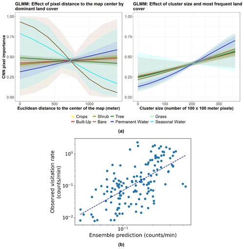
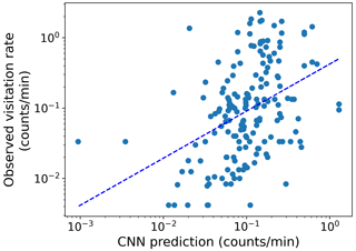
Figure 3 (a) Marginal effects of the GLMM modeling CNN pixel importance (R package ggeffects v1.3.1; Lüdecke, 2018) in Appendix C. The left subpanel shows the effect of pixel distance to the map center by “dominant land cover” on CNN pixel importance for the following land cover types: bare (brown), built-up (red), crops (yellow), grass (light green), permanent water (dark blue), seasonal water (cyan), shrub (olive), and tree (dark green). The right subpanel displays the effect of the cluster size (to which the pixel belongs) and the most frequent land cover type of that cluster on CNN pixel importance for the same land cover types. Lines represent expected values of explanatory variables, and bands represent confidence intervals. (b) The observed visitation rate (counts per minute) versus the predicted visitation rate (counts per minute) using the ensemble model for bumblebees and other wild bees combined. The dashed line shows a linear fit. The Spearman rank correlation value obtained is S_ρ=0.64.

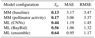
Regarding our second hypothesis, which posited that a model based on land cover maps with more complex rules would outperform the mechanistic models in Giménez-García et al. (2023), the CNN model achieved a global rank correlation coefficient of 0.44 for pollinator visitation rates, roughly doubling the best mechanistic model (0.17, Table 1, Figs. 2 and E1). Simple mechanistic rules like those in Lonsdorf et al. (2009) could perform reasonably well in homogeneous (simple) landscapes but less effectively in heterogeneous (complex) landscapes (Kennedy et al., 2013), where our approach can be better suited.

Additionally, our findings confirm our third hypothesis: CNNs enhance the predictions of previous data-driven models without land cover maps. Our ensemble model improved the rank correlation from 0.56 to 0.64 (Table 1, Figs. 2 and 3b). While we are still far from achieving a high predictive power at global scales, as more data become available, these modeling techniques hold promise not only to predict pollinator ecosystem services, but also to interpret which landscape characteristics are explaining these predictions.

Table 1 Metrics obtained by comparing predictions and observations from different models on a global scale: Spearman's coefficient (S_ρ), mean absolute error (MAE), and root-mean-square error (RMSE). The mechanistic models (denoted by MM) are tested for the taxonomical group of other wild bees globally under two configurations: the baseline by Lonsdorf et al. (2009) and the configuration that considers pollinator activity (see Giménez-García et al., 2023, for further details). The data-driven models (denoted by ML for “machine learning”) are applied to the combined data from two taxonomical groups: bumblebees and other wild bees (BayRid denotes Bayesian ridge regressor). Bold characters indicate variables with a p value <0.05.

Not only do we confirm that data-driven models can help us identify important variables in ecological services such as pollination (Civantos-Gómez et al., 2021; Gardner et al., 2020), but also their ability to uncover non-obvious patterns in data, such as maps, may also enhance our mechanistic understanding of these services in environments that are data-rich but lack expert biome-specific knowledge (Borowiec et al., 2022). The challenge lies in developing strategies to increase the interpretability of deep learning algorithms so that experts can assess data-inferred prediction rules, providing the best opportunity to obtain realistic representations of complex ecological processes like pollination. Deep learning, serving as both an alternative and a complement to mechanistic modeling in solving complex inference problems, is poised to become a crucial tool for efficiently using managed pollinators and supporting wild pollinator populations in agricultural landscapes.

Appendix A: Description of the convolutional neural network model

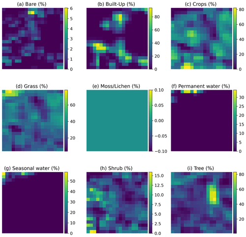
Figure A1 Example of the inputs per site fed into the convolutional neural network. Each input is a tensor with nine layers and 19 × 19 pixels. Each layer, represented as a panel in the figure, corresponds to one of the nine fraction maps, providing proportional estimates (i.e., the percentage of a 100 m pixel covered by a specific class of land cover) for vegetation and ground cover types: bare (a), built-up (b), crops (c), grass (d), moss/lichen (e), permanent water (f), seasonal water (g), shrub (h), and tree (i). The color bars show the proportional estimate of each land cover type. The data are extracted from the Dynamic Land Cover product, which provides annual global land cover maps and cover fraction layers for the reference years 2015 to 2019 (Buchhorn et al., 2020).

We developed a CNN model to predict wild-bee visitation rates, a continuous output value, based on annual global land cover maps. The model's structure, sketched in Fig. 1, is as follows:

• Input layers. Each input consists of a tensor with nine layers and 19×19 pixels. Each layer represents one of the nine fraction maps, which provide proportional estimates (i.e., the percentage of a 100 m pixel covered by a specific land cover class, namely bare cover, built-up, crops, grass, moss/lichen, permanent water, seasonal water, shrubs, and trees). These maps are derived from the Dynamic Land Cover product, which offers annual global land cover maps and cover fraction layers for the reference years 2015 to 2019 (Buchhorn et al., 2020) (see Fig. A1 for an example of the inputs).

• Convolutional layers. The model has six convolutional layers.

  The first layer processes the nine input layers using 16 filters, each with a kernel size of 3 × 3, a stride of 1, and padding of 1. This setup means each filter looks at a 3 × 3 area of the input, moving 1 pixel at a time (stride), and padding ensures the output size is the same as the input size. This results in 16 feature maps. Each feature map represents the response of the filters to the input, indicating the activation level of specific neurons within the network. For example, Fig. A2 shows the feature maps extracted from the first layer of our CNN model for the input displayed in Fig. A1. These feature maps capture basic elements such as edges, boundaries, and corners. The second layer takes the previous 16 feature maps and applies 32 filters (kernel size: 3 × 3; stride: 1; padding: 1) to create 32 new feature maps, detecting more complex patterns. The third, fourth, fifth, and sixth layers apply 64, 128, 256, and 512 filters (kernel size: 3 × 3; stride: 1; padding: 1), respectively.

  After each convolutional layer, a SELU (scaled exponential linear unit) function is applied (Klambauer et al., 2017). This function introduces non-linearity, helping the network learn more complex patterns.

• Output layer. After the final convolutional layer, the output is flattened, converting the 2D feature maps into a 1D vector. This vector is then fed into the final part of the network, which processes the combined information to produce the final output, the predicted visitation rate.

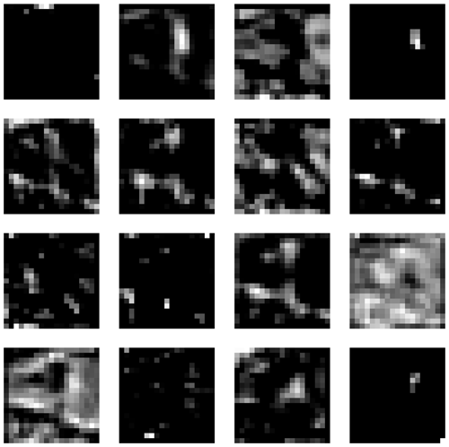
Figure A2 Feature maps extracted from the first layer of our CNN model for the input shown in Fig. A1.

We used PyTorch (Paszke et al., 2019) for fitting the convolutional neural network. In this training process, the model uses the mean-squared-error loss function to measure the difference between predicted and actual values. We trained the model for 1000 epochs using the AdamW optimizer (Loshchilov and Hutter, 2019) with a learning rate of 0.001 and a weight decay of 0.0001 to prevent overfitting. Additionally, L2 regularization is applied with a factor of 0.01, manually computed, and added to the loss to further penalize large weights and reduce overfitting.

Appendix B: Results on pixel importance for the CNN model

To create visual explanations for our predictions, we adapted the Gradient-weighted Class Activation Mapping (grad-CAM) technique by (Selvaraju et al., 2019) to our regressor CNN. This technique helps us understand which parts of the image the CNN focuses on when predicting the visitation rates of wild bees, highlighting the most important areas. Specifically, grad-CAM generates an activation map by taking a weighted sum of the feature maps from the final convolutional layer of the CNN. These weights are determined by the regressor, indicating which features are most influential in predicting the visitation rates. The importance (grad-CAM) values are normalized between 0 and 1, with higher values indicating greater importance. For instance, the importance values for the land cover types in Fig. A1 are shown in Fig. B1. When analyzing the 19 × 19 pixel input maps from the test dataset, we found that 68.6 % of the pixels are not considered important (grad-CAM = 0; see histogram in Fig. B2).

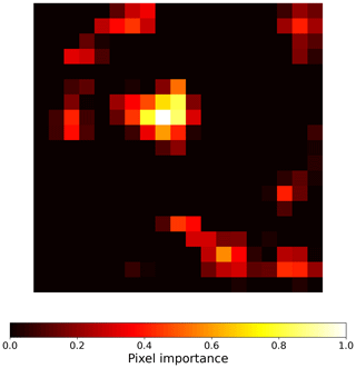
Figure B1 Activation map generated in the sixth convolutional layer of the convolutional neural network model for the input shown in Fig. A1. The heatmap visualizes the pixels that are most important for the model's decision, highlighting the regions that contribute the most to the prediction of a specific visitation rate. The importance values are normalized between 0 and 1, where higher importance is represented by brighter colors and lower importance (closer to zero) is represented by darker colors.

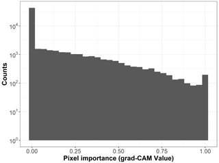
Figure B2 Histogram of the pixel importance (grad-CAM value) for the 19 × 19 pixel input maps (n=170 sites).

To facilitate the interpretation of the importance that grad-CAM assigns to each pixel, we first created a map representing the dominant land cover for each pixel. Then we used the grad-CAM values to define the transparency of the map's pixels: less important pixels appear faded, while highly important pixels retain almost their original color. For example, Fig. B3a shows the dominant land cover map for the area in Fig. A1, and Fig. B3b displays the result of applying grad-CAM transparency to the same image. This approach allows us to gain visual insights into the specific regions and their dominant land cover that are critical for identifying the visitation rate of wild bees. Additionally, we identified the Euclidean distance of each pixel to the center of the map, the size of clusters of pixels considered important (grad-CAM value > 0), and the most frequent dominant land cover within each cluster (MF-LC). As an example, Fig. B3c shows the different clusters that appear in Fig. B3b.

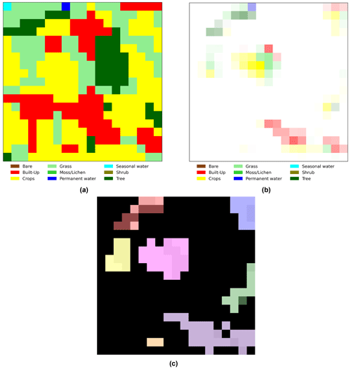
Figure B3 (a) Example of the “dominant land cover map” where each pixel is assigned the land cover type with the highest proportional estimate, as illustrated in Fig. A1. (b) Result of applying grad-CAM transparency in Fig. B1 to the map in panel (a). Less important pixels appear faded, while highly important pixels retain almost their original color. (c) Clusters of important pixels (grad-CAM value > 0) that appeared when processing the map in Fig. A1 (n=7 clusters).

Our dataset contained 61 370 pixels from 19 × 19 pixel input maps (n=170 sites). The dominant land cover type for most pixels was crops (41.7 %), followed by trees (28.7 %), grass (16.6 %), and built-up areas (9.9 %). There were no pixels where moss/lichen cover was dominant.

Overall, the pixels were at a medium distance from the center of the maps (726.09±269.78 m on average) and belonged to clusters with highly variable sizes (206.11±97.75 pixels per cluster on average). Most of these clusters were dominated by the aforementioned land cover types: crops (47.8 %), trees (29.8 %), grass (15.7 %), and built-up areas (6.6 %).

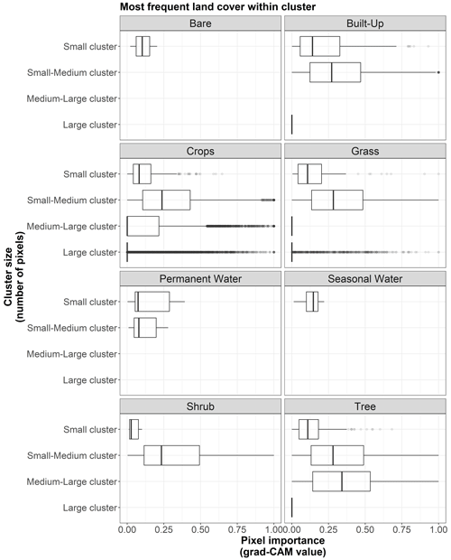
We show the pixel importance for each pixel of the 170 test sites at different levels of the following variables: (i) the dominant land cover within the pixel (Fig. B4), (ii) the Euclidean distance of each pixel to the center of the map (Fig. B5), (iii) the most frequent land cover within the cluster where the pixel belongs (Fig. B6), and (iv) cluster size (Fig. B7).

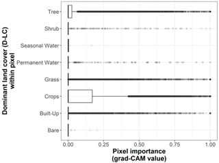
Figure B4 Box plots displaying pixel importance (grad-CAM value) for each dominant land cover type within the 19 × 19 pixel input maps from the test dataset (n=170 sites): bare, built-up, crops, grass, moss/lichen, permanent water, seasonal water, shrub, and tree.

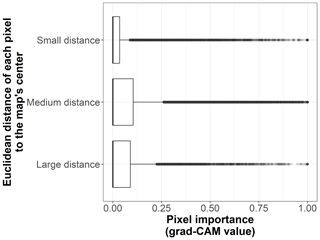
Figure B5 Box plots displaying pixel importance (grad-CAM value) in relation to the Euclidean distance of each pixel to the center of the map, for the 19 × 19 pixel input maps from the test dataset (n=170 sites). The distance categories are small (up to 500 m), medium (between 500 and 1000 m), and large (more than 1000 m).

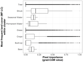
Figure B6 Box plots displaying pixel importance (grad-CAM value) for the most frequent land cover types within clusters of the 19 × 19 pixel input maps from the test dataset (n=170 sites): bare, built-up, crops, grass, moss/lichen, permanent water, seasonal water, shrub, and tree.

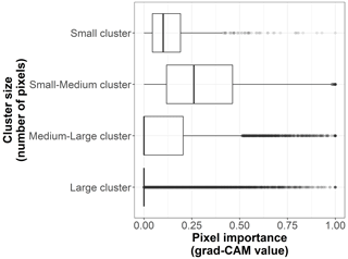
Figure B7 Box plots displaying pixel importance (grad-CAM value) for the cluster sizes of the 19 × 19 pixel input maps from the test dataset (n=170 sites). The size categories are small (up to 5 pixels), small–medium (6 to 100 pixels), medium–large (101 to 200 pixels), and large (more than 200 pixels).

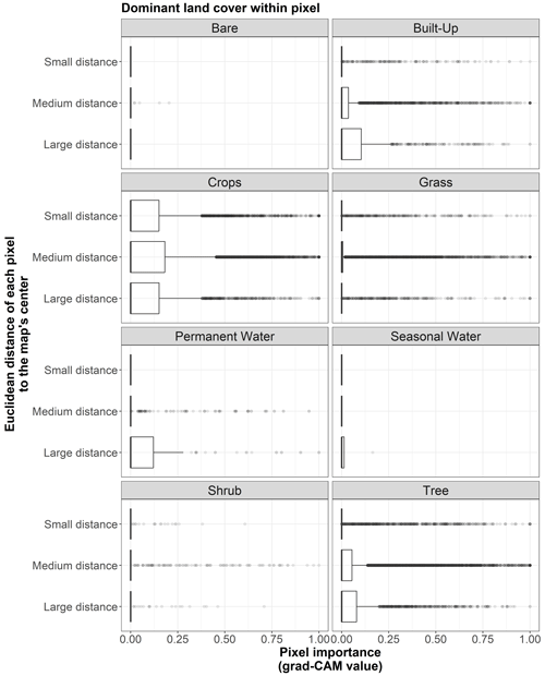
Figure B8 Box plots displaying pixel importance (grad-CAM value) in relation to the Euclidean distance of each pixel to the center of the map, categorized by the dominant land cover within each pixel. The distance categories are those displayed in Fig. B5.

Figure B9 Box plots displaying pixel importance (grad-CAM value) for the cluster sizes of input maps based on the most frequent land cover (MF-LC) within each cluster. The size categories are those displayed in Fig. B7.

Appendix C: Modeling pixel importance

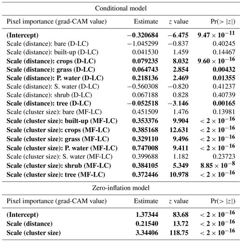
Table C1 Results for the following zero-inflated beta GLMM (n=61 370 pixels): pixel importance ∼ (interaction between pixel's distance to the map's center (distance) and its dominant land cover (D-LC)) + (interaction between the cluster size (size) and most frequent land cover within the cluster (MF-LC)) + (1|site). The hurdle model depends on distance and cluster size. Bold characters indicate variables with p value <0.05. “P. water” and “S. water” denote “permanent water” and “seasonal water”, respectively.

C1 Model for pixel importance

To explore how land cover composition and configuration affect the importance of a given pixel, we fitted a general linear mixed model (GLMM) to each pixel of the 19 × 19 land cover maps of the test dataset. We used the pixel's grad-CAM value as our response variable, and, given that we are considering zero-inflated data at the unit interval (Fig. B2), we used a zero-inflated beta regression model. The model included the following as explanatory variables: (i) the interaction between a pixel's dominant land cover (D-LC) and its distance to the center of the map and (ii) the interaction between the cluster size where the pixel belongs and the most frequent land cover within that cluster (MF-LC). The size of the cluster and the most frequent land cover within that cluster cannot be included simultaneously as explanatory variables due to high collinearity. We used “site” (i.e., the map ID) as a random intercept to account for multiple pixels within the map of each site. To fit the zero-inflation model we considered the distance to the center of the map and the size of the cluster as explanatory variables.

To keep the regression variables on similar scales and to use the fitted parameters of the models as (within-study) effect sizes, i.e., measures of variable importance (Schielzeth, 2010), all numeric explanatory variables were centered and scaled during the analysis.

Our analyses were conducted in R v4.3.0 (R Core Team, 2021), with the glmmTMB v1.1.9 package (Brooks et al., 2017). We found no high collinearity among explanatory variables when we checked their variance inflation factors with the R package performance v0.8.0 (Lüdecke et al., 2020). We also checked model assumptions with the R package DHARMa v0.4.6 (Hartig, 2020).

Figure C1 DHARMa diagnostics for the zero-inflated beta GLMM, when the full dataset is considered (sample n=61 370 pixels; “KS test” denotes “Kolmogorov–Smirnov test”) (Hartig, 2020).

Figure C2 DHARMa diagnostics for the zero-inflated beta GLMM, considering only a randomly selected subset of the full dataset (sample n=6000 pixels; n.s. denotes “not significant”) (Hartig, 2020).

C2 Model results

The model results are shown in Table C1. According to the zero-inflation model, the probability of a pixel having zero importance and not being part of the original uninflated beta distribution significantly increases for pixels that are far away from the center of the map (distance ⪆ 726 m) and for those pixels that belong to very large clusters (cluster size ⪆ 206 pixels).

Regarding the conditional model, after controlling for variation at the site level, our findings show that important pixels (grad-CAM > 0) dominated by trees tend to be significantly more important when they are closer to the center of the map (where the visitation rate is measured). In contrast, important pixels mainly covered by crops, grass, or permanent water (grad-CAM > 0) increase in importance when they are located farther from the center of the map.

Additionally, important pixels that belong to clusters most frequently covered by built-up areas, crops, grass, permanent water, shrubs, and trees tend to be more important in larger clusters. However, it should be noted that, according to Fig. B9, clusters dominated by built-up areas, permanent water, and shrubs tend to be smaller than average.

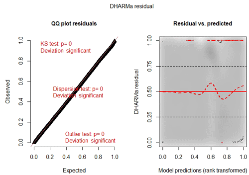
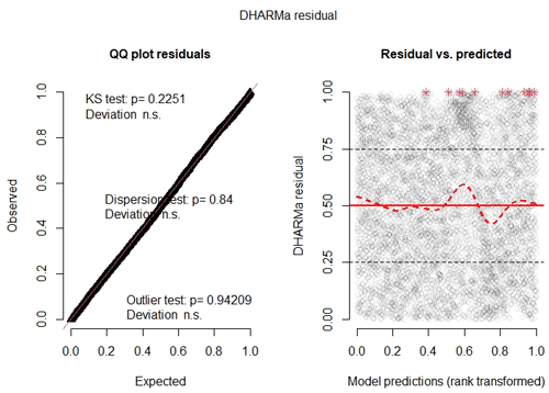
Finally, upon examining the model's residuals and assumptions, we found that their distribution cannot be perfectly described by a beta distribution (Fig. C1). This is primarily due to the large sample size (n=61 370 pixels). An analysis of the same zero-inflated beta GLMM fitted to a random 10 % subsample of the dataset shows better agreement with the modeling assumptions (Fig. C2), and the trends of the coefficients are similar to those of the model fitted with the complete data (table not shown). Nevertheless, since the model is used only to interpret pixel importance and not for making predictions, the results of the full model are considered valid.

Appendix D: Ensemble (stacking) model

We developed a fully connected neural network (FCNN) model to predict wild-bee visitation rates, a continuous output value, based on the predictions from the best machine learning model in Giménez-García et al. (2023), the Bayesian ridge regressor. The model's structure (model 3 in Fig. D1) is as follows:

• Input layer. The input to the network is a tensor representing the predictions obtained from the CNN model (Appendix A) and those from the best machine learning model in Giménez-García et al. (2023).

• Hidden layers with batch normalization and dropout. The model consists of two hidden layers with batch normalization and dropout, designed to improve training stability and prevent overfitting.

  • First hidden layer. The first hidden layer is a fully connected (dense) layer with 32 neurons. After the linear transformation, batch normalization is applied to normalize the output of the linear layer. This is followed by a ReLU (rectified linear unit) activation function to introduce non-linearity. Dropout with a rate of 0.685 is then applied, randomly setting one-third of the activations to zero during training to prevent overfitting.

  • Second hidden layer. The second hidden layer is also a fully connected layer with 32 neurons. Similarly to the process for the first hidden layer, batch normalization is applied, followed by the ReLU activation function and dropout with a rate of 0.685.

• Output layer. The final layer is a fully connected layer with a single neuron, which produces the predicted visitation rate. Since the task is regression, no activation function is applied at this stage, allowing the output to be any real number.

The model was implemented using PyTorch (Paszke et al., 2019) and trained using the model NeuralNetRegressor from the skorch library. The training process involved the following settings:

• Loss function. Mean-squared-error (MSE) loss was used to measure the difference between predicted and actual values.

• Optimizer. The Adam optimizer (Loshchilov and Hutter, 2019) was employed with a learning rate of 0.1.

• Training duration. The model was trained for 50 epochs.

• Data shuffling. Training data were shuffled at the beginning of each epoch to ensure the model did not learn the order of the training examples.

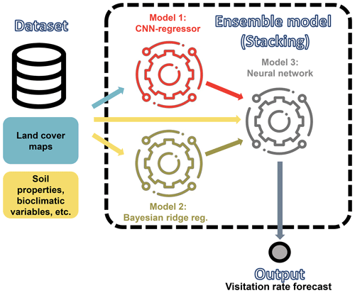
Figure D1 Schematic representation of our ensemble model to predict visitation rates of wild bees. The algorithm is fed with the inputs required to run the CNN model shown in Fig. 1 and the best machine learning model identified by Giménez-García et al. (2023), the Bayesian ridge regressor. The ensemble model employs a neural network to estimate the visitation rates of wild bees using the predictions from these models.

Appendix E: Results at a global scale for the CNN model

Figure E1 The observed visitation rate (counts per minute) versus the predicted visitation rate (counts per minute) using the CNN model for bumblebees and other wild bees combined. The dashed lines show a linear fit. The Spearman rank correlation value obtained is S_ρ=0.44.