Geographically weighted models in palaeoecology: R package and application to testate amoebae in peatlands

Transfer function (TF) models are commonly used in palaeoecology for quantitative inference of environmental variables based on biological proxies. Although the existence of spatial structure is well established in ecology, existing TFs do not account for it. This suggests that model performance may be improved by accounting for spatial structure. Here we demonstrate this using basic and advanced methods – multiple linear regression (MLR), lasso regression, geographically weighted regression (GWR) and geographically weighted lasso (GWL) – using geographical distance and bioclimatic distance, respectively. We compared the performance of these models for reconstructing water table depth from testate amoeba communities, as commonly used in peatland palaeoecology. GWL and lasso models performed considerably better (23 %–30 % reduction in mean squared prediction error) than standard weighted average methods. We provide an R package for the two innovative spatial methods (GWR and GWL).

1 Introduction

Understanding how ecosystems responded to past environmental change is fundamental to determining how to manage or restore them in the context of ongoing environmental change (Seddon et al., 2014; Swetnam et al., 1999). A wide range of methods are used in palaeoecology to reconstruct past changes in environmental conditions or ecosystem functioning. Key drivers such as temperature or soil moisture are often inferred from biotic proxies (e.g. (sub-)fossil pollen, diatoms and testate amoebae) using mathematical models called “transfer functions” (Birks et al., 1990).

Aquatic or terrestrial microorganisms, especially protists, are ideal proxies for environmental monitoring and palaeoecological inference. They are abundant, diverse, sensitive to variations in (micro)environmental conditions over time or space, and directly involved in key ecosystem processes such as carbon cycling (Payne, 2013). Some groups, such as diatoms and testate amoebae, produce decay-resistant structures (“shells”, called frustules or tests in these two groups, respectively) that can be recovered from peat or sediments (Harnisch, 1927; Tolonen, 1987; Warner, 1990). This makes it possible to document changes in community structure over time and, if the relationships between community structure and environmental conditions are known, to infer past environmental changes from these changes. The key to such reconstructions is the development of accurate inference models calibrated on modern data (the so-called training set).

The presumed cosmopolitan distribution of microorganisms (O’Malley, 2008; De Wit and Bouvier, 2006) was considered an advantage for the development of transfer functions. Indeed, if microbes do not vary in space, it is likely that the ecological preference of species is also constant over time (i.e. the uniformitarian principle) (Hutton, 1788). However, it is becoming increasingly clear that not all microorganisms are cosmopolitan (Seppey et al., 2020; Foissner, 2006; Telford et al., 2006), implying that the spatial component of the data needs to be integrated into model development (Belyea, 2007; Payne et al., 2012). However, this bias is rarely, if ever, considered when attempting to build transfer function models over large geographical areas (Amesbury et al., 2016, 2018; Qin et al., 2021). Improving palaeoecological reconstructions based on microorganisms therefore requires better knowledge of microbial diversity, ecology and distribution, as well as advances in the mathematical methods used to develop predictive models. Mathematical improvements include seeking for more appropriate models (weighted average, maximum likelihood calibration, partial least squares, etc.), selecting species (e.g., removing rare or taxonomically uncertain taxa) and accounting for spatial distribution (e.g., using one-site-out cross-validation) (Payne et al., 2012; Juggins and Birks, 2012).

In this study, we aim to develop and test novel mathematical models that account for spatial structure to infer past environmental conditions from biotic proxies. We use testate amoeba (TA)-based models which are primarily used to infer past water table depth (WTD) in peatlands (Charman, 2001; Mitchell et al., 2008).

2 Material and methods

We compare four types of regression model with the model developed by Amesbury et al. (2016), which is used as a reference. Amesbury's model (the best-performing model with a root mean squared prediction error (RMSEP) of 10.87 before outlier removal) is called WA-Tol (inv), which stands for “Weighted Averaging with Tolerance downweighting and Inverse deshrinking”. It relies on the assumption that each taxon has an ecological optimum and that if a taxon is very abundant in a fossil sample, the ecological parameter to be inferred in this fossil sample should be close to the optimum of the modern taxon. Tolerance downweighting is applied to give less weight to taxa that have a large ecological tolerance (their ecological optimum for the investigated parameter is broad). Inverse deshrinking is then applied to the model to compensate for compression of variance due to the weighing average procedure. In our study, all models are tested on the same dataset. The different regression models and the dataset are presented below.

2.1 Models

2.1.1 Multiple linear regression (MLR)

A MLR (see, for instance, Quinn and Keough, 2023) is a linear regression with p independent variables $x_{\mathrm{1}},x_{\mathrm{2}},\mathrm{\dots },x_p$:

$$\begin{array}{}\text{(1)}& y_i={\mathit{\beta }}_{\mathrm{0}}+\sum _{k=\mathrm{1}}^p{\mathit{\beta }}_k{x}_{ik}+{\mathit{ϵ}}_i,\end{array}$$

where y_i is the response variable for observation i (with $i=\mathrm{1},\mathrm{2},\mathrm{\dots },n$), n is the total number of observations, β₀ is the intercept, β_k is the kth regression coefficient for variable x_k (with k in $\mathrm{1},\mathrm{2},\mathrm{\dots },p$), p is the total number of explanatory variables, x_ik represents the k explanatory variables of observation i, and $i\sim N(\mathrm{0},{\mathit{\sigma }}^{\mathrm{2}})$ is the error term for observation i; all the error terms are independent.

The models’ parameters $\mathrm{0},\mathrm{\dots },p$ are usually estimated using the ordinary least squares (OLS) method; i.e. regression coefficients are estimated by minimising the sum of the squared prediction errors:

$$\begin{array}{}\text{(2)}& {\widehat{\mathit{\beta }}}_{\mathrm{OLS}}=\underset{\mathit{\beta }}{min}\left\{\sum _{i=\mathrm{1}}^n{\left(y_i-{\mathit{\beta }}_{\mathrm{0}}-\sum _{k=\mathrm{1}}^p{\mathit{\beta }}_k{x}_{ik}\right)}^{\mathrm{2}}\right\},\end{array}$$

where ${\widehat{\mathit{\beta }}}_{\mathrm{OLS}}$ is the vector of estimated regression coefficients ${\mathit{\beta }}_{\mathrm{0}},\mathrm{\dots },\mathit{\beta }p$.

However, the OLS method suffers from two major problems: high variance of the estimates leading to imprecision in predictions and a lack of parsimony (all variables are included even if they are not pertinent) (Tibshirani, 1996).

2.1.2 Lasso regression

The lasso (least absolute shrinkage and selection operator) regression (Tibshirani, 1996) solves both problems of MLR by adding a constraint on the sum of the absolute value of the regression coefficients:

$$\begin{array}{}\text{(3)}& {\widehat{\mathit{\beta }}}_{\mathrm{L}}=\underset{\mathit{\beta }}{min}\left\{\sum _{i=\mathrm{1}}^n{\left(y_i-{\mathit{\beta }}_{\mathrm{0}}-\sum _{k=\mathrm{1}}^p{\mathit{\beta }}_k{x}_{ik}\right)}^{\mathrm{2}}+{\mathit{\lambda }}_{\mathrm{L}}\sum _{k=\mathrm{1}}^p\left|{\mathit{\beta }}_k\right|\right\},\end{array}$$

where λ_L is the lasso regularisation penalty parameter.

Hence, the lasso stabilises the coefficients, reducing their variance, and performs variable selection by setting some coefficients to zero, resulting in a parsimonious model. This type of model is typically used to handle genetic data with many explanatory variables (Ranstam and Cook, 2018).

However, MLR as well as lasso are both global regression models; i.e., they assume spatial homogeneity and estimate one fixed regression coefficient for each predictor. The purpose of our research here is to integrate spatial heterogeneity, meaning the heterogeneous distribution of microorganisms (explanatory variables) when estimating an environmental parameter (response variable), so we introduce geographically weighted models.

2.1.3 Geographically weighted regression (GWR)

The principle of GWR is to fit a local MLR for each observation (Brunsdon et al., 1996; Fotheringham et al., 2002). Therefore, regression coefficients are not fixed but vary according to the geographical locations for each variable. The collection of local models then forms a global model:

$$\begin{array}{}\text{(4)}& y_i={\mathit{\beta }}_{\mathrm{0}}(u_i,v_i)+\sum _{k=\mathrm{1}}^p{\mathit{\beta }}_k(u_i,v_i)x_{ik}+{\mathit{ϵ}}_i,\end{array}$$

where β₀(u_i,v_i) and β_k(u_i,v_i) are the local regression coefficients at location (u_i,v_i).

As regression coefficients are estimated at each observation’s location, each of them is characterised by three numbers: the coordinates (latitude, longitude) and its estimated value. When fitting a local regression on a point of interest (an observation), we only consider its closest neighbours. To select them, we use a distance matrix (usually based on the Euclidean distance). The threshold distance from the point in which we consider the neighbours is called bandwidth and is chosen by cross-validation. The optimal bandwidth is the one that minimises the prediction error. Weights are attributed to the neighbours based on their distance to the point and a kernel function. The kernel function usually attributes a higher weight to closer neighbours and a lower weight to farther ones. The weights are then directly used in the regression to estimate the β regression coefficients by weighted least squares:

$$\begin{array}{}\text{(5)}& {\widehat{\mathit{\beta }}}_{\mathrm{GWR}}(u_i,v_i)=\left({\mathbf{X}}^{\mathrm{T}}\mathbf{W}\right(u_i,v_i\left)\mathbf{X}{)}^{-\mathrm{1}}{\mathbf{X}}^{\mathrm{T}}\mathbf{W}\right(u_i,v_i)\mathit{Y},\end{array}$$

where X is an n×p explanatory variable matrix with n the total number of observations and p the total number of explanatory variables; W(u_i,v_i) is an n×n diagonal weight matrix for location (u_i,v_i), with $\mathbf{W}(u_i,v_i)=\mathrm{diag}\left(K_h\right(d_{i\mathrm{1}},K_h(d_{i\mathrm{2}},\mathrm{\dots },K_h(d_{in}\left)\right)\left)\right)$; K_h is the kernel; d_ij is the distance between observations i and j (with $j=\mathrm{1},\mathrm{\dots },n$); and Y is a vector of n response variables.

There are several possible kernel shapes divided into two categories: continuous kernels (Fig. 1a) and kernels with compact support (Fig. 1b). In the first category, we find uniform, Gaussian and exponential kernels; in the second we find boxcar, bisquare and tricube kernels. Kernels with compact support are usually preferred as they ease calculation, since all weights beyond a fixed bound are set to zero (De Bellefon and Loonis, 2018).

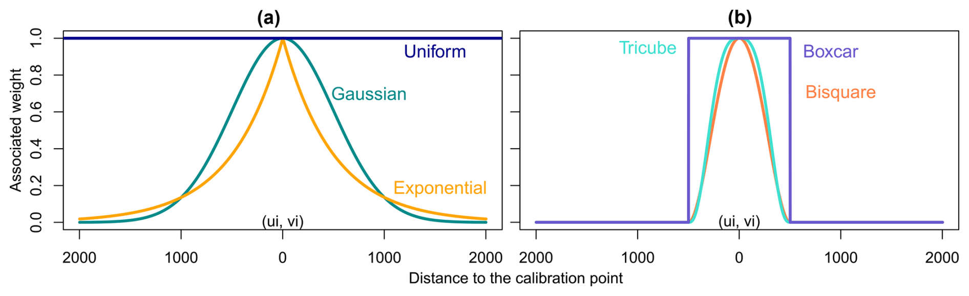
Figure 1 Different kernel shapes. (a) Continuous kernels: they are defined over the whole domain but do not reach zero; (b) compact kernels: they are defined over the whole domain but are set to zero outside a fixed range.

The kernel can be fixed or adaptive depending on what defines its extent. If it is determined by a fixed distance to the point of interest, the kernel is identical at any location and is considered fixed (Fig. 2a). On the other hand, if the kernel’s extent is determined by the number of neighbours to consider, the kernel will be large when there is a low observation density and small when density is high; we call it an adaptive kernel (Fig. 2b).

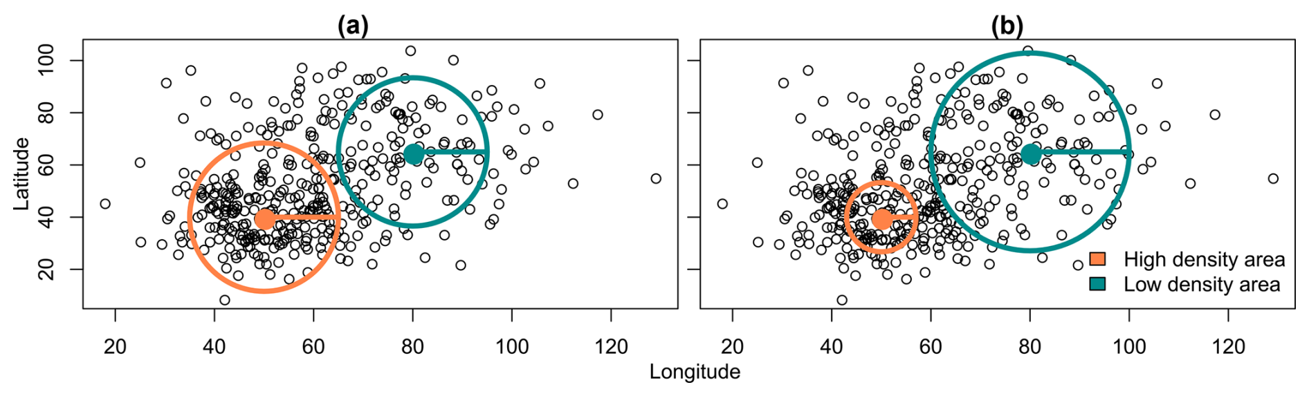
Figure 2 Two kernel configurations. (a) Fixed kernel: the distance does not vary; (b) adaptive kernel: the distance varies according to the density.

2.1.4 Geographically weighted lasso (GWL)

GWR models are already improved versions of MLR as they take into account local variations. However, local correlation in explanatory variables can lead GWR to estimate strongly correlated regression coefficients, which is problematic for inference on relationship between variables (Wheeler and Tiefelsdorf, 2005). With respect to local correlation, three phenomena must be considered: pairwise variables' correlation (or collinearity), multicollinearity and spatial autocorrelation (SA). Pairwise correlation is well known, but multicollinearity and spatial autocorrelation are often ignored. Multicollinearity appears when some explanatory variables of a dataset, in a MLR, are linked by a linear relation, i.e. when one can be reconstructed based on the others. And spatial autocorrelation, similarly to temporal autocorrelation where two observations close in time tend to have correlated values, occurs when geographically close observations have similar values. To model relationships in a dataset presenting local correlation, we recommend the use of GWL, which is more robust to local correlation (Wheeler, 2009). The lasso, by adding a constraint on the magnitude of the estimated coefficients, stabilises the coefficients and limits the effects of correlation of the explanatory variables.

$$\begin{array}{}\text{(6)}& \begin{array}{rl}{\widehat{\mathit{\beta }}}_{\mathbf{GWL}}(u_i,v_i)& =\underset{\mathit{\beta }}{min}\left\{\sum _{i=\mathrm{1}}^n{\left(y_i-{\mathit{\beta }}_{\mathrm{0}}(u_i,v_i)-\sum _{k=\mathrm{1}}^p{\mathit{\beta }}_k(u_i,v_i)x_{ik}\right)}^{\mathrm{2}}\right.\\ & \left.+{\mathit{\lambda }}_{\mathrm{GWL}}\sum _{k=\mathrm{1}}^p\left|{\mathit{\beta }}_k(u_i,v_i)\right|\right\},\end{array}\end{array}$$

where λ_GWL is the GWL regularisation penalty parameter.

Therefore, in addition to considering the spatial structure, GWL has the advantage of producing a parsimonious model as lasso regression performs variable selection. GWL models have been used for various applications; for example, Wang and Zuo (2020) applied GWL to detect geochemical anomalies by identifying geological parameters that are locally significant, and Im and Kim (2021) used such a model to identify local socio-economic factors that enhanced the transmission of SARS-CoV-2 in the Seoul metropolitan area during the COVID-19 pandemic.

2.2 Dataset

In this work, we use a dataset published in Amesbury et al. (2016) (called “Amesbury” in our R package; see Sect. 5). That study aimed to build a pan-European transfer function using the most common reconstruction models (WA, weighted averaging partial least squares regression (WA-PLS), maximum likelihood (ML) and MAT) along with a large geographically extended dataset, spanning from Spain to western Russia. This large dataset is a compilation of several datasets. The details of this compilation and the exhaustive list of datasets included are given in Amesbury et al. (2016). The compiled dataset contains 1799 samples from 113 sites in 18 countries. Each sample is characterised by four descriptive variables (PERSON (the analyst), COUNTRY, SITE, SAMPLE), two geographical coordinates (Lat (latitude), Long (longitude)) and 62 numerical measures (WTD (water table depth), pH and the relative abundances of 60 taxa). In total, the dataset contains 68 variables.

We worked on the cleaned dataset, the same used as input in the article of Amesbury et al. (2016). To clean it, the authors made a few changes: to begin with, due to the large number of contributors in the compiled dataset, the authors adopted a low-resolution taxonomy to unify the data. Morphologically similar taxa were merged to form new groups (morpho-taxa). The rationale is that (1) TA with a similar shape likely share similar ecological preferences and (2) morphologically similar taxa are more likely to be misidentified, potentially leading to erroneous inference (Payne et al., 2011) – pooling them reduces this bias (but also the precision). Rare taxa were removed, as well as samples with “NA” values, and high pH value and extreme WTD measurements were removed as they risk distorting the prediction. Finally, the cleaned dataset included 1103 samples and 47 taxa, resulting in 55 variables in total. For model fitting, we only used WTD, the coordinates (Lat, Long) and the 47 taxa.

2.3 Model comparison

To assess the performance of the GWL method, we calculated its root mean squared prediction error (RMSEP) using the leave-one-out (LOO) technique and compared it with the RMSEP of other models (Birks, 2003). In total, we compared seven different models based on their prediction error (see Table 1): MLR, lasso, two GWR models (GWR-geo and GWR-bio, using geographical and bioclimatic distance, respectively, for spatial selection), two GWL models (GWL-geo and GWL-bio, similar to GWR), and WA-Tol (inv) as a reference. WA-Tol (inv) stands for “Weighted Averaging with Tolerance downweighting and Inverse deshrinking” and is the best-performing model in Amesbury et al. (2016). For GWR and GWL models, we used the Euclidean geographical and bioclimatic distances. Bioclimatic data were retrieved from the CHELSA database (Karger et al., 2018, 2017).

Two steps are required to fit a geographically weighted model: (1) calculating the optimal bandwidth through cross-validation and (2) fitting local models using the previously calculated bandwidth for neighbour selection. Due to computational limitations, we calculated the optimal bandwidth for each geographically weighted method (GWR-geo, GWR-bio, GWL-geo, GWL-bio) once for each model instead of once for each LOO step, and we used the same bandwidth for all LOO steps. We checked the validity of this assumption by calculating the bandwidth for each LOO step of a subset of 500 observations from the original dataset. As the 500 bandwidth values were very stable (mean = 1062, sd = 0), we concluded that this assumption was reasonable in regard to computational time savings.

3 Results

The results of calculating the RMSEP for each of the six models and for Amesbury's model are shown in Table 1, together with the bandwidths (n nearest neighbours selected for local regression) for the geographically weighted models. The order of the models corresponds to their description in Sect. 2.1, with the reference model coming first, and the others listed in order of increasing recency. The RMSEP expresses the mean prediction error in centimetres (cm) in predicting the WTD, so a smaller RMSEP indicates better performance. The ranking of the models, from best to worst in terms of prediction error, is the following: GWL-geo, lasso, GWR-geo, MLR, GWL-bio, GWR-bio and finally Amesbury's WA-Tol.

Table 1 Performance of different regression models for inferring the water table depth from testate amoeba communities.

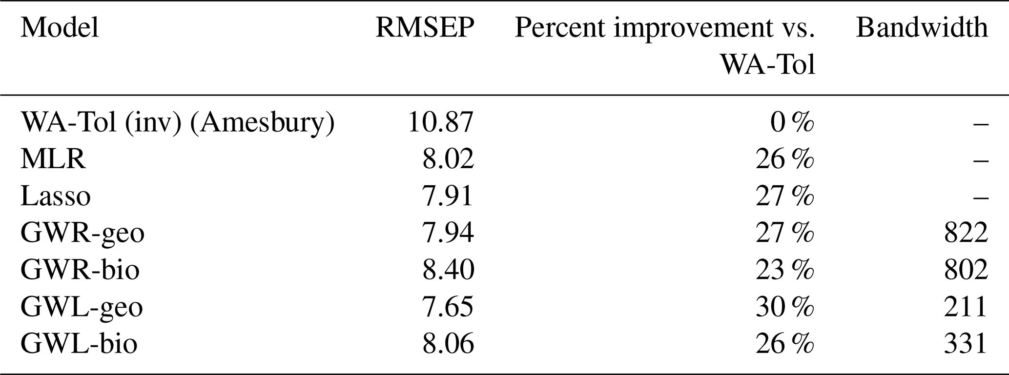
All models performed substantially better than Amesbury's WA-Tol model. Geographically weighted models provide a 27 % and 30 % improvement in model performance as assessed using RMSEP, while the improvement using bioclimatic weighted models is somewhat lower (23 % and 26 %). In contrast, the differences in RMSEP between lasso, GWR and GWL models are small (at most 0.75 cm between GWR-bio and GWL-geo). Compared to Amesbury, our GWL-geo model, the best-performing model, improves the reconstruction with a gain of 3.22 cm (30 % improvement) in accuracy, which is considerable relative to the range of WTD values we predict.

The bandwidths also provide information on the selective behaviour of the geographically weighted models. The GWL models are more parsimonious in terms of the number of neighbours selected for the local regressions, selecting 19 % and 30 % of the observations (n=1103) as neighbours for GWL-geo and GWL-bio, respectively. GWR, on the other hand, is much less local, selecting 74 % and 73 % of the observations as neighbours for GWR-geo and GWR-bio, respectively.

In addition to improving prediction, geographically weighted models, particularly GWL, allow for the production of maps of the importance of each species (explanatory variable) by location. Since geographically weighted models fit local regressions, we obtain local regression coefficients that can be interpreted as the influence of the species on the prediction of WTD at a given location. A coefficient close to zero indicates that the presence of the species is not informative to predict the WTD, while the presence of a species with non-null coefficients indicates wetter conditions if the coefficient is negative (higher WTD) and drier conditions if the coefficient is positive (lower WTD). The map therefore indicates in which region a species should or should not be considered. For example, Fig. 3 illustrates the importance of Arcella discoides (ARC.DIS), a taxon associated with wet conditions. We note that it is important to consider in northern Europe, especially in Ireland and the UK, but not in central Europe, where its coefficients are almost null. In this sense, species with null coefficients in most locations are poor indicators.

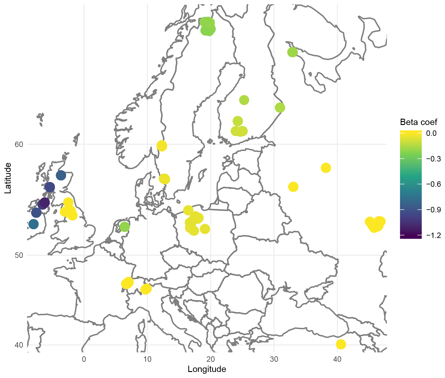
Figure 3 Map of the β regression coefficients for Arcella discoides (ARC.DIS), according to each location extracted from the GWL model based on geographical distance.

4 Discussion

Given the existence of spatial structure in ecology, we hypothesised that the performance of the testate amoeba water table depth transfer function model would improve if models incorporated geographic or bioclimatic information. Our results clearly confirm this hypothesis, with up to 30 % improvement in model performance compared to the model presented by Amesbury et al. (2016). Furthermore, we found that the performance of basic methods such as lasso and MLR is surprisingly good compared to spatially aware models. The respectable performance of the lasso model also highlights that this dataset, with many explanatory variables, is likely to be too noisy for other models that do not perform variable selection. In this context, the advantages of GWL are confirmed: spatial awareness, robustness to correlation (multicollinearity, autocorrelation) and variable selection. On the one hand, GWL-geo, the best-performing model, allows one to characterise the importance of a species depending on the location, but on the other hand, it is computationally intensive compared to the lasso model, which also performs well. We therefore suggest choosing between these two methods depending on the objective of the study: using a lasso for a simple reconstruction when we focus on predicting the WTD in a relatively restricted area and using a GWL when we focus not only on prediction but also on characterising the bioindicator value of species in a wider area.

Nonetheless, our results using this dataset (maps and regression coefficients) must be considered with caution due to the nature of the dataset. Indeed, the dataset is a compilation, and different authors contributed data from different regions, so there may be a potentially significant and geographically structured identification bias. The grouping of species reduces this bias but still introduces a problem of low taxonomic resolution, as the newly defined “morpho-taxa” have broader ecological preferences and thus a loss of specificity. A possible solution and future work would be to consider morphological traits instead of species or taxa, as they may be better indicators of the living conditions of microorganisms (Fournier et al., 2015; Marcisz et al., 2020).

5 R package

To allow researchers to use GWL, typically for palaeoreconstruction, we published an R package called “GWlasso” (Mulot and Erb, 2024). The package also includes the dataset we used in this study, which is presented in Sect. 2.2. In general, we do not recommend the use of GWR models, especially for biological objects, due to their sensitivity to local correlation (Wheeler, 2009). For this reason, we did not include them in the package.

To fit a GWL model, two steps are necessary: first calculate the optimal bandwidth (bw) parameter through cross-validation with function gwl_bw_estimation and, second, use the optimal bandwidth to fit the model with function gwl_fit(). The inputs for the bandwidth and fitting functions are similar: a matrix of explanatory variables (x.var), a vector of corresponding response variable (y.var), a matrix of distance between observations (dist.mat) and a few parameters to specify the model’s local selection criteria (kernel type, adaptive or not). In addition, function gwl_bw_estimation requires the smallest bandwidth to be tested (adaptbw.thresh), and gwl_fit() requires a bandwidth value, ideally the optimal bandwidth calculated with the corresponding bandwidth function.

Further documentation is available in the dedicated GitHub repository (Mulot and Erb, 2024). Our code is inspired by “Geographically weighted elastic net logistic regression” from Comber and Harris (2018) for the spatial selection of neighbours.

6 Conclusions

Despite some caveats, the relative differences between Amesbury’s model and our new models are solid results as they only report the change in model performance using the same input. Those results suggest reconsidering the actual reconstruction models commonly used in palaeoecology, and they explore the use of more recent mathematical methods, like GWL and lasso models, in this field. The GWL method already has applications in socio-economics (Setiyorini et al., 2017) and geochemistry (Wang and Zuo, 2020) but, to our knowledge, not yet in ecology, and it seems to be promising. Future work using this method is now needed.