An approach to the modeling of honey bee colonies

In this work, populations of adult and immature honeybees and their honey production are studied through mathematical and statistical modeling approaches. Those models are complementary and are presented in disjunct form. They were used to show different modeling methods for honey bee population dynamics. The statistical approach consisted of a generalized linear model using data from the Department of Agriculture of the United States of America (USDA), which showed that the relationship between the number of colonies and the rate of honey production is not constant in time but decrease over the years. These models showed that when a bee population is subjected to a stress factor (i.e., habitat destruction, Varroa mite, climate variability, season, neonicotinoids, among others), the abundance of individuals decreases over time as well as the honey produced by the colonies. Finally, the mathematical approach consisted of two models: (1) a smooth model, in which conditions of existence and stability of the equilibrium solutions are determined by an ecological threshold value, and (2) a non-smooth model where the mortality rate of bees is included as a function of the number of adult bees in the population.

1 Introduction

Bees are one of the most ecologically and commercially important insects in the world (Brown and Paxton, 2009). There are approximately 20 000 species of bees (Nates-Parra, 2011), from which Apis mellifera is the most common for commercial purposes (Hardstone and Scott, 2010). Bees are of great importance not only for humans, but also for all plant species that they pollinate. The most important crops around the world are visited and pollinated by bees and rely on them for reproduction (Patel et al., 2021). In tropical crops, 70 % of the 1330 cultivated species are favored by these pollinators, while in European crops, 84 % of the 264 cultivated species depend on the animal pollination process, and it is known that the yields of some fruit, seed and nut crops decrease by more than 90 % without these pollinators (García et al., 2016; Klein et al., 2007; Garibaldi et al., 2012).

Bees also contribute to the maintenance of native ecosystems, because pollination helps to regenerate trees, which help to conserve forest biodiversity, as well as preserving other ecosystem services (Nates-Parra, 2016). This makes bees important regulators of food production, forest balance and micro-climate dynamics (Winfree, 2010). From all species of bees, only a few are eusocial; Apis mellifera is an example of eusocial behavior (Woodard et al., 2011). This species forms colonies so that the survival, reproduction and honey production depend on the structure and size of the colonies (Mattila and Seeley, 2007).

Honey is a sweet natural substance produced by honeybees using mainly the nectar of flowers, which is transformed by a group of enzymes present in the saliva of the worker bees, which is also airy and evaporates by its fluttering, and is finally stored inside the hives of the nest. Honey from Apis mellifera is one of the most important zoo-agricultural goods for commercial trade in the world (Campos and Leyva, 2018; Ulloa et al., 2010; Farouk et al., 2014). The utility of honey is diverse. For example, it works as an anti-flu agent (Farouk et al., 2014). Honey also serves as a natural source of antioxidants which are effective in reducing the risk of heart and immune system diseases, cataracts and various inflammatory symptoms (Vit, 2004). Regarding the honey trade, the United States of America is the world leader in imports. Honey imports increased at a rate of 6956 t yr⁻¹, making this country the main honey importer in the world (García, 2018). However, regarding production, China is the world leader (466.6 kt), followed by Turkey (94.7 kt), Iran (74.6 kt), Ukraine (73.7 kt) and the Russian Federation (68.4 kt) (Güngör, 2018).

Despite the great importance of bees in the world, an alarming concern has been raised in the last 20 years because of the decrease in the number of honey bees worldwide, which affects the quality of life of all human populations that depend (directly or indirectly) on them (Ratnieks and Carreck, 2010; Cox-Foster and VanEngelsdorp, 2009; Nates-Parra, 2016).

For these reasons, it is necessary to develop studies on honey bee population dynamics aiming to conserve and sustainably manage this species. Research in the area of mathematics and statistics has contributed to the development of models that allow us to understand the population dynamics of bee colonies (Belić et al., 1986; Schmickl and Crailsheim, 2008; Khoury et al., 2011; Russell et al., 2013; Jatulan et al., 2015; Dennis and Kemp, 2016; Booton et al., 2017). Schmickl and Crailsheim (2007) created a simple mathematical bee population model (HoPoMo) using differential equations to predict the population dynamics and resource fluctuations of a bee colony. Their model emphasized the importance of pollen supply (Bagheri and Mirzaie, 2019) and presented a mathematical model considering pollen and nectar as necessary foods for the colony. This model was developed based on the differential equations proposed by Khoury et al. (2013). Schmickl and Crailsheim (2007) built one of the most detailed population models of honey bee colony dynamics, consisting of 60 equations that track the life of a bee from an egg to an adult bee every day. The model considered the effect of seasonal changes in egg-laying rate, nurse bees on larval survival and pollen shortage on cannibalization. Russell et al. (2013) developed a model that focused on how internal demographic processes within a colony interact with food availability and brood rearing to alter growth in forager population size. The model was implemented as a series of differential equations based on the rate equations from the analytical models proposed by Khoury et al. (2013).

In this work, we describe from mathematical and statistical perspectives the relationship between the population size of honey bees (Apis mellifera) and honey production when the bee colony is subjected to some stress factor (habitat destruction, climatic variability, neonicotinoids, etc.) that externally causes the death of individuals and consequently the possible decrease in honey production. We present three different approaches. Two of them are purely mathematical and consider the interaction between immature and adult bees and the amount of honey produced using ordinary differential equations (ODEs).

First, we consider a smooth model in which a stability analysis of the equilibrium solutions is performed. The stability results are validated with numerical experiments using data obtained from the literature. Next, we consider a non-smooth model which is analyzed using Filippov's systems theory (Dieci and Lopez, 2009). Finally, a statistical model is developed considering honey production as the response variable, the number of colonies as a the main effect predictor, and year, latitude and area as covariates, using a generalized linear model (GLM).

2 The statistical model approach

For this section, we used the historical data of bee farming in the United States of America (USA) from 1985 to 2019, from the US Department of Agriculture (USDA), which are publicly available on USDA web page (https://usda.library.cornell.edu/concern/publications/hd76s004z?locale=en&page=3#release-items, last access: August 2022). Additionally, for a detailed revision, the R codes and the cleaned data set are available at the following GitHub link: https://github.com/jpatirom3/Honey-bees-modeling- (last access: March 2022). These data sets summarize the statistics of honey production and number of bee colonies by state and year in the USA. We used these data sets because they offer the most complete, comprehensive and publicly available data on honey production in the world. After checking the data sets for missing data, we decided to use the data from 39 states, which had complete values for all years.

A first exploration of these data sets revealed a significant decreasing trend in honey production over the years (Fig. 1), which is an expected pattern due to the worldwide decrease of working honeybees during the last 20 years (Bretagnolle and Gaba, 2015). Since this kind of temporal trend can inflate the relationship between responses and predictors in statistical models (Wooldridge, 2015), we fitted a model for each of seven 5-year sub-series (1985–1989, 1990–1994, 1995–1999, 2000–2004, 2005–2009, 2010–2014 and 2015–2019), in such a way that the temporal trend within each sub-series was significantly reduced in comparison to the full 1986–2019 series. Thus, every model was able to be built on n=194 data points, which is a reliable sample size for parameter estimation. This approach also allowed us to evaluate the temporal change of the parameters over time, which is important due to the already mentioned decline of bees.

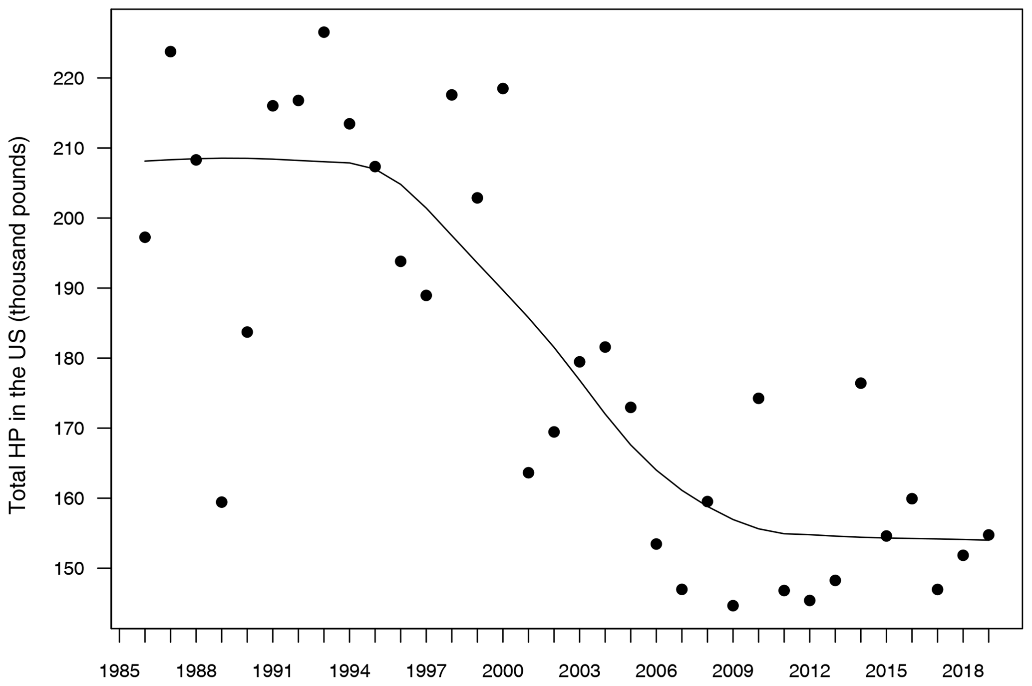
Figure 1 Evolution of total honey production in the USA from 1985 to 2019. Units in the y axis are shown as thousand pounds. The solid line represents a temporal trend fitted by a locally weighted polynomial regression.

Thus, our modeling approach considered honey production (HP) (pounds) as the response variable for each of the seven 5-year sub-series; number of colonies (NC) as the main effect predictor; and year (Y), latitude (LAT) and area (AR) (hectares) of each state as covariates. Since NC and HP exhibited highly skewed distributions, we used an additive GLM log–log with a logged response and predictor in order to achieve normal and homoscedastic residuals (Quinn and Keough, 2002). Equation (1) shows the specification of this model, where e is an error term with Gaussian distribution and Id is an identity link function.

$$\begin{array}{}\text{(1)}& \mathrm{Id}(\mathrm{logHP}{)}_{i=\mathrm{1}}^{\mathrm{7}}={\mathit{\beta }}_{\mathrm{1}}+{\mathit{\beta }}_{\mathrm{2}}(\mathrm{logNC})+{\mathit{\beta }}_{\mathrm{3}}Y+{\mathit{\beta }}_{\mathrm{4}}\mathrm{LAT}+{\mathit{\beta }}_{\mathrm{5}}\mathrm{AR}+e\end{array}$$

Estimation of β parameters was performed trough the iterative reweighted least squares method (IWLS) (Stirling, 1984). Different combinations of covariates were fitted in a top-down stepwise modeling approach, which started by fitting a saturated model with all covariates and ended up with a reduced final model with a minimum number of covariates that captured most of the variance in the response variable (Table 1). The Akaike information criterion (AIC) and the root mean square error (RMSE) were used as metrics of performance and prediction accuracy to compare among models and define the final models for each year's sub-series. β₂, of main interest for this section, was interpreted as a percentage unit change in HP caused by a percentage unit change in NC, while keeping the other covariates parameters constant. All these procedures were done in R studio (R Team, 2019).

Table 1 Results of analysis of deviance for the statistical models fitted to the data for every 5-year sub-series. Residual deviance represents the degree in which the response variable can be predicted by model predictors. The higher the value, the better the model is able to make predictions. The F value is the rate of model variance; it provides a way to compare the fitted model against a model with only intercept and no predictors. Higher F values represent better fits of the data to the model. F values provide the significance of the effect of each predictor in the models. Values equal to or lower than 0.05 represent a significant effect. R² is the coefficient of determination; it represents the percentage of variance in the response variable that is explained by the fitted model.

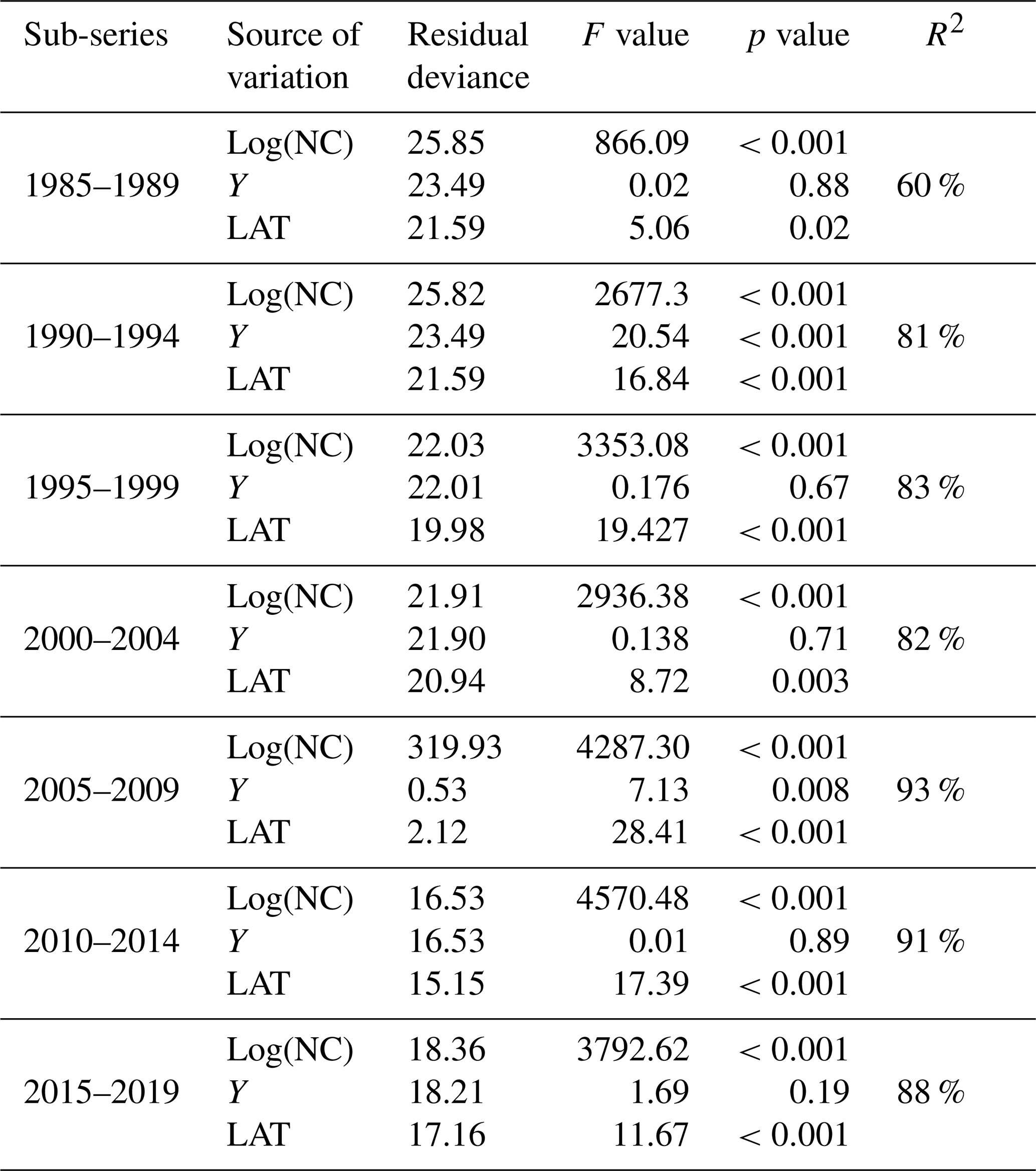
Table 1 shows the results of the statistical modeling processes in terms of analysis of deviance. Covariates in the final reduced models were Y and LAT. AR was dropped because AIC values did not decrease in any of the models that included it. Figure 2 shows the predicted values of the models as a function of NC and HP. In general, the performance and prediction accuracy of all models were satisfactory, since R² ranged between 60 % and 93 %. Parameter estimation showed that β₂, of main interest for our study, reduced over the years from 1.14±(0.06) in 1985–1989 to 1.05±(0.02) in 2014–2019 (Fig. 3) (values in brackets represent 95 % confidence intervals). This is a reduction of 8 % in the effect of NC on HP. These values can be interpreted in such a way that during 1985–1989, a 1 % increase in NC caused an increase of 1.1 % to 1.14 % in HP, whilst in 2014–2019, a 1 % increase in NC caused an increase of 1.03 % to 1.07 % in HP.

Figure 2 Real HP (honey production) values (black solid dots) and predicted HP values (red open circles) from GLMs plotted against real NC values in logarithmic scale for the seven sub-series of years.

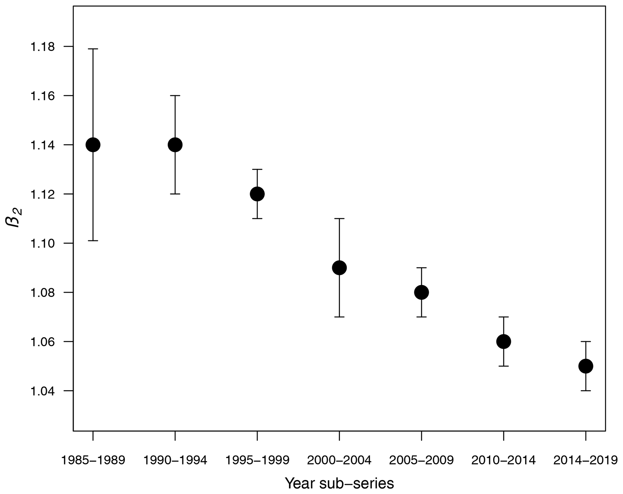
Figure 3 Decay of β₂ over the years. Vertical bars represent 95 % confidence intervals estimated from GLMs.

Figure 4 Honey bee and food dynamics represented in the model (Eq. 5). Dashed lines represent food consumption and mortality.

3 The smooth mathematical model approach

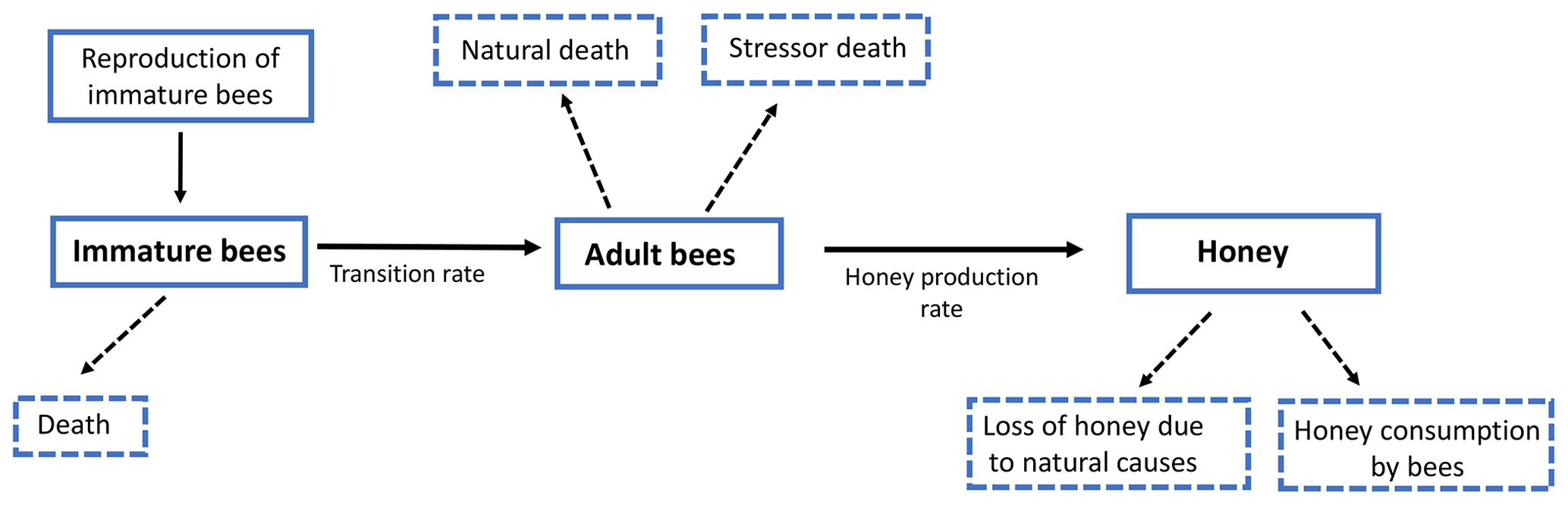
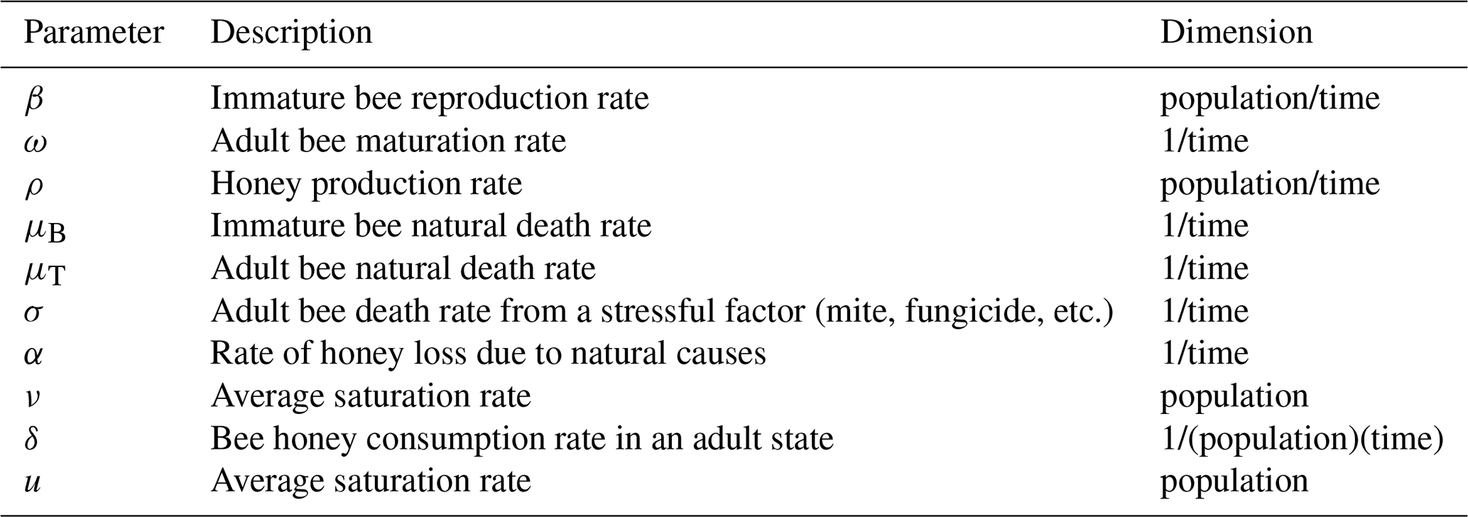
In this section we formulate a smooth mathematical model that describes the interaction among immature bees at time t(B(t)), adult bees at time t(T(t)) and the amount of honey produced at time t(M(t)). We assumed that immature bees grow at a rate β, proportionally to the number of adult bees. This is represented by term $T/(T+\mathit{\nu })$, where ν is the average saturation rate (number of adult bees needed for immature bees to reach the half of its maximum number). The number of bees reaching the adult stage affects the number of immature bees. This is modeled by term ωB, where ω represents the maturation rate to the adult stage, and $\mathrm{1}/\mathit{\omega }$ represents the time spent before reaching the adult state. Additionally, the number of immature bees is reduced by natural mortality. This is modeled by term μ_BB, where μ_B represents the natural death rate of the immature stage. In this way, the following ODE is proposed to model the variation in the number of immature bees at time t:

$$\begin{array}{}\text{(2)}& {\displaystyle \frac{\mathrm{d}B}{\mathrm{d}t}}=\mathit{\beta }{\displaystyle \frac{T}{T+\mathit{\nu }}}-\mathit{\omega }B-{\mathit{\mu }}_{\mathrm{B}}B.\end{array}$$

Similarly, we assumed that the number of adult bees decreases naturally. This is represented by term μ_TT, where μ_T is the natural death rate of the adult stage. Additionally, the bees can also die due to a stress factor. This was modeled by the term σT, where σ is the death rate due to a stress factor (loss of habitat, pesticides, climate change, mismanagement by the beekeeper, among others) on bees at the adult stage. Thus, the number of adult bees at time t can be represented by the following ODE:

$$\begin{array}{}\text{(3)}& {\displaystyle \frac{\mathrm{d}T}{\mathrm{d}t}}=\mathit{\omega }B-{\mathit{\mu }}_{\mathrm{T}}T-\mathit{\sigma }T.\end{array}$$

Finally, the production of honey in the hives increases at a rate ρ, which depends on the number of adult bees. This is represented by the term $T/(T+u)$, where u is the average saturation rate. The amount of produced honey decreases due to different factors; one of them is the loss of honey due to natural causes such as support for the hive and feeding of immature bees, which is represented by the term αM, where α is the rate of honey loss. Another cause is the consumption by adult bees, which is modeled by term δTM, where δ is the rate of honey consumption by adult bees. Therefore, the following ODE models the variation in the proportion of existing honey at time t:

$$\begin{array}{}\text{(4)}& {\displaystyle \frac{\mathrm{d}M}{\mathrm{d}t}}=\mathit{\rho }{\displaystyle \frac{T}{T+u}}-\mathit{\alpha }M-\mathit{\delta }TM.\end{array}$$

From Eqs. (2)–(4) we obtain the following system of ODEs:

$$\begin{array}{}\text{(5)}& \left\{\begin{array}{ll}\frac{\mathrm{d}B}{\mathrm{d}t}& =\mathit{\beta }\frac{T}{T+\mathit{\nu }}-\mathit{\omega }B-{\mathit{\mu }}_{\mathrm{B}}B\\ \frac{\mathrm{d}T}{\mathrm{d}t}& =\mathit{\omega }B-{\mathit{\mu }}_{\mathrm{T}}T-\mathit{\sigma }T\\ \frac{\mathrm{d}M}{\mathrm{d}t}& =\mathit{\rho }\frac{T}{T+u}-\mathit{\alpha }M-\mathit{\delta }TM\end{array}\right..\end{array}$$

Model (Eq. 5) can be represented in Fig. 4.

The specifications of parameters involved in the model (Eq. 5) are shown in Table 2.

Table 2 Parameters involved in the model (Eq. 5): description and dimension.

Let us define $\mathit{ϵ}=\min \mathit{\{}{\mathit{\mu }}_{\mathrm{B}},{\mathit{\mu }}_{\mathrm{T}}\mathit{\}}$. Then, the set of biological interest of the model (Eq. 5) is given by

$$\begin{array}{}\text{(6)}& \mathrm{\Omega }=\left\{(B,T,M)\in {\mathbb{R}}_{+}^{\mathrm{3}}:\mathrm{0}\le B+T\le {\displaystyle \frac{\mathit{\beta }}{\mathit{ϵ}}},\mathrm{0}\le M\le {\displaystyle \frac{\mathit{\rho }}{\mathit{\alpha }}}\right\}.\end{array}$$

The following lemma ensures that set Ω has biological sense; that is, all solutions starting in Ω remain there for all t≥0.

Lema 3.1. The set Ω defined in Eq. (6) is positively invariant for the solutions of the system (Eq. 5).

The proof of the above lema can be seen in Appendix A.

3.1 Equilibrium points

For calculating the equilibrium points and stability of the model (Eq. 5), it should be clarified that all parameters given in Table 2 are strictly greater than zero. The equilibrium points of the system (Eq. 5) are given for the solution of the following system of algebraic equations

$$\begin{array}{}\text{(7)}& \left\{\begin{array}{l}\mathrm{0}=\mathit{\beta }\frac{T}{T+\mathit{\nu }}-\mathit{\omega }B-{\mathit{\mu }}_{\mathrm{B}}B\\ \mathrm{0}=\mathit{\omega }B-{\mathit{\mu }}_{\mathrm{T}}T-\mathit{\sigma }T\\ \mathrm{0}=\mathit{\rho }\frac{T}{T+u}-\mathit{\alpha }M-\mathit{\delta }TM\end{array}\right..\end{array}$$

Details about the solution of the previous system can be found in Appendix A. We get the following proposition.

Proposition 3.2. Model (Eq. 5) always has a trivial equilibrium ${\mathbf{E}}_{\mathrm{0}}=(\mathrm{0},\mathrm{0},\mathrm{0})$. Besides, if ${\mathit{\lambda }}^{*}>\mathit{\nu }$ there is a non-trivial equilibrium ${\mathbf{E}}_{\mathrm{1}}=(b^{*},{\mathit{\lambda }}^{*}-\mathit{\nu },m^{*})$, where b^* and m^* are defined in Eqs. (A4) and (A5), respectively.

3.2 Local stability analysis

Here, we determine the conditions for the local stability of the equilibrium solutions given in Proposition 3.2. We use the linearization of the vector field given by the right-hand side of the system (Eq. 5), which is given by the following Jacobian matrix:

$$\begin{array}{}\text{(8)}& \mathbf{J}\left(\mathbf{E}\right)=\left(\begin{array}{lll}-\left(\mathit{\omega }+{\mathit{\mu }}_{\mathrm{B}}\right)& \frac{\mathit{\beta }\mathit{\nu }}{(T+\mathit{\nu }{)}^{\mathrm{2}}}& \mathrm{0}\\ \mathit{\omega }& -\left({\mathit{\mu }}_{\mathrm{T}}+\mathit{\sigma }\right)& \mathrm{0}\\ \mathrm{0}& \frac{\mathit{\rho }u}{(T+u{)}^{\mathrm{2}}}-\mathit{\delta }M& -(\mathit{\alpha }+\mathit{\delta }T)\end{array}\right).\end{array}$$

The stability of each equilibrium point given on Proposition 3.2 can be found by evaluating the above matrix in each equilibrium point. To see the mathematical details see Appendix A. We obtain the following proposition.

Proposition 3.3. If ${\mathit{\lambda }}^{*}<\mathit{\nu }$, the trivial equilibrium ${\mathbf{E}}_{\mathrm{0}}=(\mathrm{0},\mathrm{0},\mathrm{0})$ is locally and asymptotically stable, whereas if ${\mathit{\lambda }}^{*}>\mathit{\nu }$, it is unstable. If ${\mathit{\lambda }}^{*}=\mathit{\nu }$, E₀ is a non-hyperbolic equilibrium point. Similarly, If ${\mathit{\lambda }}^{*}>\mathit{\nu }$, the coexistence equilibrium ${\mathbf{E}}_{\mathrm{1}}=(b^{*},{\mathit{\lambda }}^{*}-\mathit{\nu },m^{*})$ is locally and asymptotically stable, whereas if ${\mathit{\lambda }}^{*}<\mathit{\nu }$, it is unstable. If ${\mathit{\lambda }}^{*}=\mathit{\nu }$, E₁ is a non-hyperbolic equilibrium point.

A summary of the results from Proposition 3.3 is given in Table 3.

Table 3 Condition of the existence and stability of the equilibrium points of the model (Eq. 5).

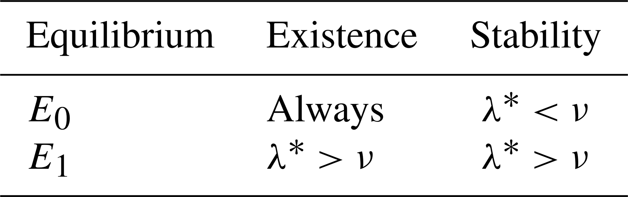
Remark 3.4. The existence and stability conditions of the equilibrium points of the system (Eq. 5) are given in terms of an ecological threshold λ^* defined in Eq. (A3), which can be rewritten as

$${\mathit{\lambda }}^{*}={\displaystyle \frac{\mathit{\omega }}{{\mathit{\mu }}_{\mathrm{T}}+\mathit{\sigma }}}*{\displaystyle \frac{\mathit{\beta }}{\mathit{\omega }+{\mathit{\mu }}_{\mathrm{B}}}}.$$

Since μ_T+σ represents the total death rate of adult bees and ω+μ_B the total death rate of immature bees, the expression $\mathit{\omega }/{\mathit{\mu }}_{\mathrm{T}}+\mathit{\sigma }$ can be interpreted as the proportion of immature bees that equals the number of adult bees when these remain constant. Similarly, $\mathit{\beta }/\mathit{\omega }+{\mathit{\mu }}_{\mathrm{B}}$ is the proportion of adult bees that equals the number of immature bees when these remain constant. Thus, λ^* is the total net number of bees produced by the colony during the lifetime of the hive. If the total death rate of adult bees is large enough, it would lead to the collapse of the hive because the term λ^* would approach to zero. This is because the existence condition of the coexistence equilibrium states that ${\mathit{\lambda }}^{*}>\mathit{\nu }$, where the constant ν is the number of adult bees required for the growth rate of immature bees to reach half its maximum value.

3.3 Numerical simulations

In this section we present some numerical experiments that illustrate the behavior of the hive and honey subjected to different parameter values. Some values were taken from the literature and others were assumed. In Table 4 we show the rank of the parameter values included in the model and their respective references.

Russell et al. (2013)Torres et al. (2015)Martínez et al. (2018)Russell et al. (2013)Russell et al. (2013)Winfree et al. (2009)Khoury et al. (2013)Brodschneider and Crailsheim (2010)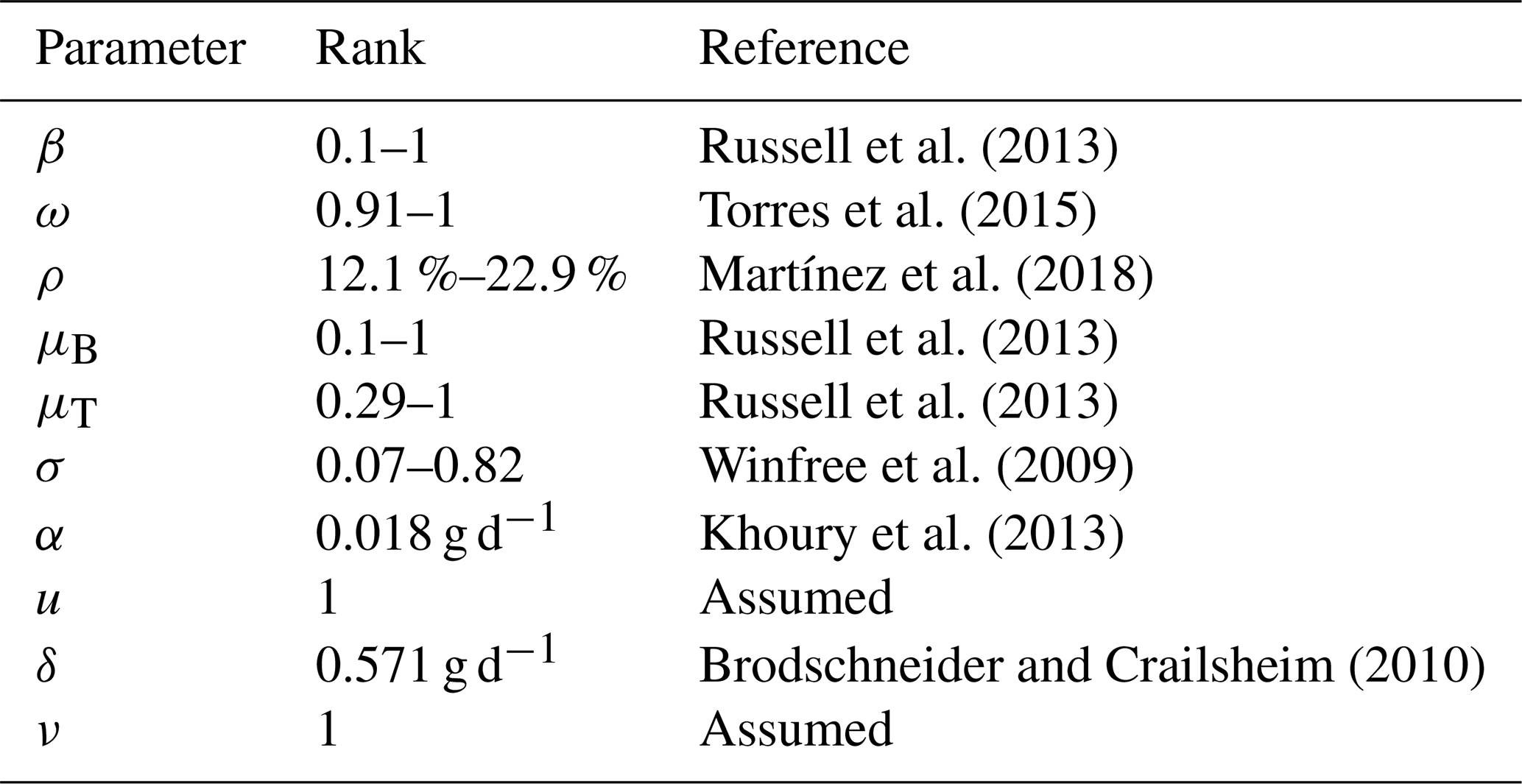

Table 4 Parameter values included in the model (Eq. 5).

In Fig. 5 we present the stability of the equilibrium E₀, which is obtained with a higher value for the reproduction rate of immature bees. Here, σ=0.8 (considered a high value), ρ=0.13, μ_B=0.11, μ_T=0.29, ω=0.95, α=0.95, δ=0.571, u=1, ν=1 and β=0.92. With these values the number of bees and their honey will constantly decrease until a collapse.

Figure 5 Numerical representation of the equilibrium E₀. Here, ${\mathit{\lambda }}^{*}=\mathrm{0.7564}$ and ν=1.

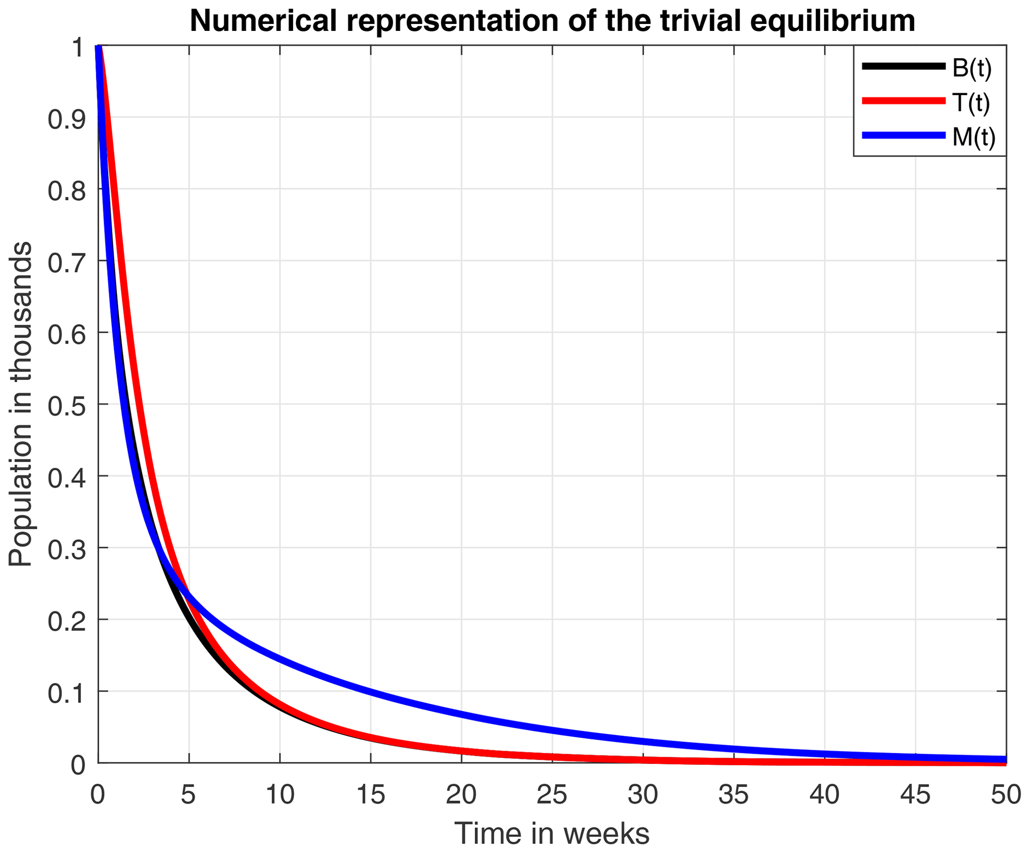
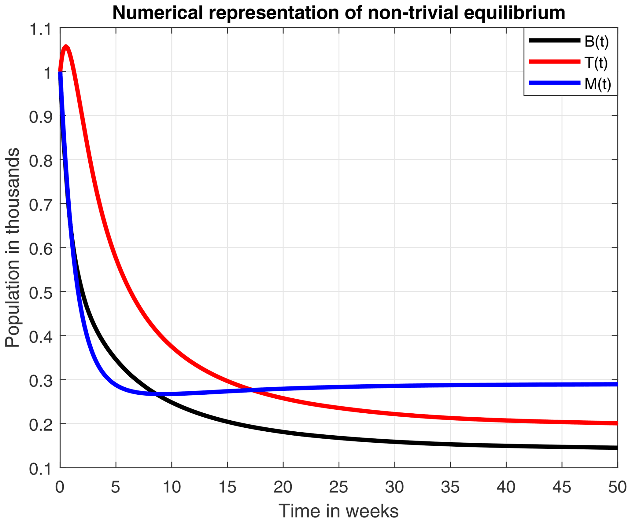
Figure 6 numerically represents the stability of the equilibrium E₁. Here, the mortality rate due to a stress factor was reduced to an average value of σ=0.4, and the honey production rate was increased to ρ=0.23. The loss of honey due to natural causes has also increased to α=0.1. By including the above changes in parameter values, the amounts of immature adults and honey production remain constant in B=0.14, T=0.2 and M=0.289. However, this is less likely to occur because, due to multiple factors, the hives tend to collapse after a certain time.

Figure 6 Numerical representation of the equilibrium E₁. Here, ${\mathit{\lambda }}^{*}=\mathrm{1.195}$ and ν=1.

4 The non-smooth mathematical model approach

Some mathematical models whose arguments are described by piecewise smooth functions have numerous dynamics and applications, as well as an extensive mathematical structure, even though their behavior is not simply described in terms of modern qualitative theory of dynamical systems. However, this classical theory of dynamic systems does not include a significant number of phenomena that occur in practice. These phenomena are defined with functions that are non-smooth in their arguments, such as electrical circuits in which there are commutations (switches), control systems, models in different sciences and population models in biology, where some continuous changes can generate discrete actions. Such is the case of bee populations, in which different stress factors can cause some thresholds of mortality and affect both the number of bees in the immature state, as well as in the adult state, and therefore honey production.

Thus, in this section we use the Filippov systems (Dieci and Lopez, 2009) to study the system (Eq. 5), where R₁ and R₂ are considered as death thresholds. If the number T of adult bees is big enough from a R₂, the death of bees due to a stress factor (σ) will be maximum (σ_max). Similarly, from a R₁, if the number of adult bees is small enough, the death rate due to a stress factor will be minimal (σ_min). Finally, if we consider that the number of adult bees is in equilibrium, that is between R₁ and R₂, the death rate due to a stress factor will be stable (σ₁). The previous consideration can be mathematically written as follows:

$$\begin{array}{}\text{(9)}& \mathit{\sigma }=\left\{\begin{array}{ll}{\mathit{\sigma }}_{\max }& \mathrm{if}T>R_{\mathrm{2}},\\ {\mathit{\sigma }}_{\mathrm{1}}& \mathrm{if}{R}_{\mathrm{1}}\le T\le R_{\mathrm{2}},\\ {\mathit{\sigma }}_{\min }& \mathrm{if}T<R_{\mathrm{1}}.\end{array}\right.\end{array}$$

The main characteristic of the Filippov systems is the subdivision of the state space into disjoint subregions, and a smooth vector field is defined within each one of them (Amador et al., 2021). The limits between the different regions are called discontinuity surfaces, which are usually denoted as Σ_i (Hogan et al., 2016).

Mathematical details about this approach can be seen in Appendix B. However, this presents only a mathematical understanding of Filippov's systems; a biological sense of this will be determined in future work, as well as the study of the presence of pseudo-equilibrium points.

4.1 Numerical simulations

The numerical simulations of this section were performed using the MATLAB interface, and the codes can be consulted at the following GitHub link: https://github.com/jpatirom3/Honey-bees-modeling- (last access: March 2022). Numerical simulations for the described systems are presented below. Figure 7 shows the trajectory of the solutions of the states B(t), T(t) and M(t). In this figure, we take B(0)=1, T(0)=1 and M(0)=1 as initial conditions. Table 5 summarizes the values used for each parameter.

Table 5 Parameter values used for numerical simulations in Figs. 7 and 8.

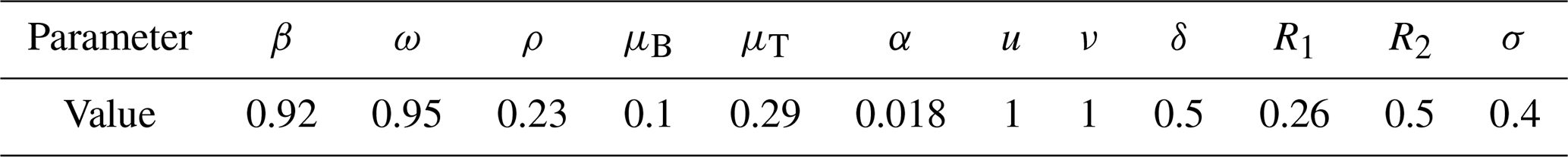
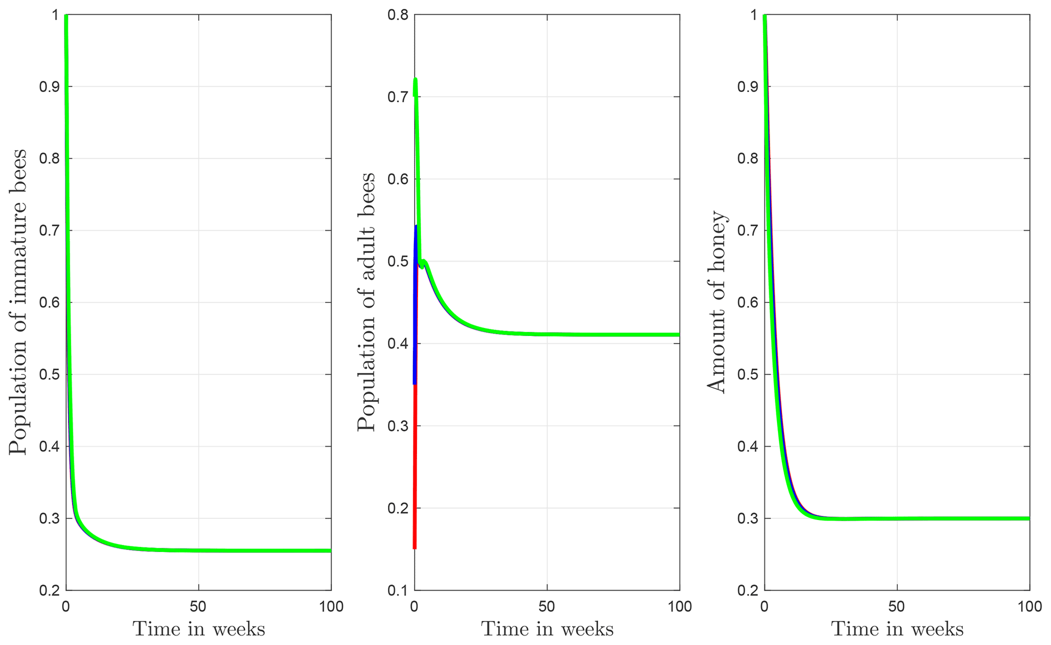
Figure 7 Trajectories for B, T and M. Here the initial condition is $\left(B\right(\mathrm{0}),T(\mathrm{0}),M(\mathrm{0}\left)\right)=(\mathrm{1},\mathrm{1},\mathrm{1})$ and β=0.9, ω=0.95, ρ=0.23, μ_B=0.1, μ_T=0.29, α=0.018, u=1, ν=1 and δ=0.5. The ecological threshold is ${\mathit{\lambda }}^{*}=\mathrm{1.2063}$.

Figure 8 Numerical simulation of the model (Eq. 9) with initial conditions – number of immature bees: 1; number of adult bees: 0.15, 0.35 and 0.7; and amount of honey: 1. The trajectories are represented by the red, blue and green curves, respectively. The parameter values are given in Table 5.

Figure 8 shows the switching surfaces Σ₁ (left side) and Σ₂ (right side), which divide the first octant into the following regions: S₁ (left side of Σ₁), S₂ (region between Σ₁ and Σ₂), and S₃ (right side of Σ₂), as well as the phase portrait. The trajectories show that regardless of the initial conditions or the region of start, there is always a crossover in the switching planes, which is proven analytically with the Filippov analysis as shown above. After some time, the trajectories remain in regions S₂ and S₃, which means that the number of adult bees is switching within these regions limited by the switching surface Σ₂. Finally, the number of adult bees seeks stability at the break-even point, as shown by Fig. 7.

5 Discussion

In this work, we attempted to contrast three different modeling approaches to understand the population dynamics of immature bees, adult bees and the honey produced in the hive. We first formulated a smooth mathematical model in which conditions of existence and stability of equilibrium solutions were found. Afterwards, we adapted the previous model to a non-smooth model which was studied using Filippov's systems theory. Finally, we analyzed a honey bee data set obtained from USDA, using a GLM.

From the smooth model, we obtained two equilibrium points: (1) a coexistence between the number of bees and honey production and (2) a collapse in both the number of bees and honey production. An important aspect to highlight here is that the existence and stability of these equilibrium points are in terms of the ecological threshold λ^*, given in Remark 3.4, which represents the net number of bees produced within the colony over the lifetime of the hive. Additionally, the numerical experiments of these two points suggested that a high death rate due to a stress factor (σ=0.8), which was used in Fig. 5, leads to a collapse of the hive in 50 weeks.

Subsequently, a smooth model was proposed in which two death thresholds R₁ and R₂ were considered for the stress factor. The Filippov analysis for the non-smooth model showed that there is always a crossover in the switching surfaces. After 100 weeks, the trajectories switched between regions S₂ and S₃, which defined a normal and high stress rate respectively, as it was shown in Fig. 8. Finally, the orbits stabilized at the equilibrium point located in region S₂. We have taken into account the fact that the equilibrium point E₁ is stable, and, therefore, the equilibrium value is reached when t→∞.

For the statistical approach, generalized linear models were built to study seven 5-year sub-series of colony abundance and honey production data (1985 to 2019) from the USDA. We observed that the number of colonies required to produce a same amount of honey is not constant but reduced over the years as shown by Fig. 3. This points to the influence of a stress factor, such as the change of natural habitats to mono-cultures (Belsky and Joshi, 2019) or the infestation by the ectoparasitic Varroa mite destructor (Guzmán-Novoa et al., 2010; Martin et al., 2012).

From these three modeling approaches, we conclude that honey production is reduced due to the decrease in the total number of bees within the colony and due to an external stress factor, which could be climate variability, pesticides, parasites such as the Varroa mite, or habitat loss, among other things. This can be observed in Fig. 6, in the simulations of the non-smooth model (Eqs. 7 and 8), and mainly in the statistical results in Fig. 3. From numerical experiments it was observed that the amount of honey produced is considerably reduced in time; however, it does not fully collapse but stay constant.

Appendix A

Proof of Lema 3.1.

Proof. It is clear that $\frac{T}{T+\mathit{\nu }}\le \mathrm{1}$. Adding the first two equations of the system (Eq. 5) we obtain

$$\begin{array}{ll}{\displaystyle \frac{\mathrm{d}(B+T)}{\mathrm{d}t}}& {\displaystyle }=\mathit{\beta }{\displaystyle \frac{T}{T+\mathit{\nu }}}-{\mathit{\mu }}_{\mathrm{B}}B-{\mathit{\mu }}_{\mathrm{T}}T-\mathit{\sigma }T\\ {\displaystyle }& {\displaystyle }\le \mathit{\beta }-{\mathit{\mu }}_{\mathrm{B}}B-{\mathit{\mu }}_{\mathrm{T}}T\\ {\displaystyle }& {\displaystyle }\le \mathit{\beta }-\mathit{ϵ}(B+T).\end{array}$$

Thus, $B+T\le \mathit{\beta }/\mathit{ϵ}$. Similarly, for M we get that

$$\begin{array}{ll}{\displaystyle \frac{\mathrm{d}M}{\mathrm{d}t}}& {\displaystyle }=\mathit{\rho }{\displaystyle \frac{T}{T+u}}-\mathit{\alpha }M-\mathit{\delta }TM.\\ {\displaystyle }& {\displaystyle }\le \mathit{\rho }-\mathit{\alpha }M-\mathit{\delta }TM\\ {\displaystyle }& {\displaystyle }\le \mathit{\rho }-\mathit{\alpha }M.\end{array}$$

Therefore, $M\le \mathit{\rho }/\mathit{\alpha }$, which concludes the proof.

A1 Equilibrium points

To solve the algebraic system given on Eq. (7), we proceed as follows.

From the second equation in Eq. (7),

$$\begin{array}{}\text{(A1)}& B=\left({\displaystyle \frac{{\mathit{\mu }}_{\mathrm{T}}+\mathit{\sigma }}{\mathit{\omega }}}\right)T.\end{array}$$

Replacing B defined in Eq. (A1) in the first equation of the system (Eq. 7) we obtain

$$T\left({\displaystyle \frac{\mathit{\beta }}{T+\mathit{\nu }}}-\left({\mathit{\mu }}_{\mathrm{T}}+\mathit{\sigma }\right)\left(\mathrm{1}+{\displaystyle \frac{{\mathit{\mu }}_{\mathrm{B}}}{\mathit{\omega }}}\right)\right)=\mathrm{0}.$$

From the previous equation we have T=0 or T≠0. First, let us suppose that T≠0, thus

$$\begin{array}{}\text{(A2)}& T={\mathit{\lambda }}^{*}-\mathit{\nu },\end{array}$$

where

$$\begin{array}{}\text{(A3)}& {\mathit{\lambda }}^{*}={\displaystyle \frac{\mathit{\omega }\mathit{\beta }}{\left({\mathit{\mu }}_{\mathrm{T}}+\mathit{\sigma }\right)\left(\mathit{\omega }+{\mathit{\mu }}_{\mathrm{B}}\right)}}.\end{array}$$

Replacing T defined on Eq. (A2) into the third equation of the system, Eq. (7), we have that

$$\mathit{\rho }{\displaystyle \frac{{\mathit{\lambda }}^{*}-\mathit{\nu }}{{\mathit{\lambda }}^{*}-\mathit{\nu }+u}}-\mathit{\alpha }M-\left({\mathit{\lambda }}^{*}-\mathit{\nu }\right)\mathit{\delta }M=\mathrm{0},$$

from where

$$\begin{array}{}\text{(A4)}& M={\displaystyle \frac{\mathit{\rho }\left({\mathit{\lambda }}^{*}-\mathit{\nu }\right)}{\left(\mathit{\alpha }+\left({\mathit{\lambda }}^{*}-\mathit{\nu }\right)\mathit{\delta }\right)\left({\mathit{\lambda }}^{*}-\mathit{\nu }-u\right)}}=:m^{*}.\end{array}$$

Now, replacing T defined on Eq. (A2) into the Eq. (A1), we obtain that

$$\begin{array}{}\text{(A5)}& B={\displaystyle \frac{\left({\mathit{\mu }}_{\mathrm{T}}+\mathit{\sigma }\right)\left({\mathit{\lambda }}^{*}-\mathit{\nu }\right)}{\mathit{\omega }}}=:b^{*}.\end{array}$$

Note that a sufficient condition for T defined in Eq. (A2), M defined in Eq. (A4) and B defined in Eq. (A5) to be positive is that ${\mathit{\lambda }}^{*}>\mathit{\nu }.$

Now, if T=0 in Eq. (A2), we obtain the trivial equilibrium solution $E_{\mathrm{0}}=(\mathrm{0},\mathrm{0},\mathrm{0})$.

A2 Local stability analysis

The stability of E₀ can be found by evaluating the above matrix in E₀. Thus,

$$\mathbf{J}\left({\mathbf{E}}_{\mathrm{0}}\right)=\left(\begin{array}{lll}-\left(\mathit{\omega }+{\mathit{\mu }}_{\mathrm{B}}\right)& \frac{\mathit{\beta }}{\mathit{\nu }}& \mathrm{0}\\ \mathit{\omega }& -\left({\mathit{\mu }}_{\mathrm{T}}+\mathit{\sigma }\right)& \mathrm{0}\\ \mathrm{0}& \frac{\mathit{\rho }}{u}& -\mathit{\alpha }\end{array}\right).$$

An eigenvalue of the previous matrix is $\mathit{\xi }=-\mathit{\alpha }$, whereas the other two eigenvalues are given by the roots of the following characteristic polynomial:

$$\begin{array}{ll}{\displaystyle }p\left(\mathit{\xi }\right)& {\displaystyle }={\mathit{\xi }}^{\mathrm{2}}+\left(\mathit{\omega }+{\mathit{\mu }}_{\mathrm{B}}+{\mathit{\mu }}_{\mathrm{T}}+\mathit{\delta }\right)\mathit{\xi }\\ {\displaystyle }& {\displaystyle }+\left[\left(\mathit{\omega }+{\mathit{\mu }}_{\mathrm{B}}\right)\left({\mathit{\mu }}_{\mathrm{T}}+\mathit{\delta }\right)-{\displaystyle \frac{\mathit{\omega }\mathit{\beta }}{\mathit{\nu }}}\right]\\ {\displaystyle }& {\displaystyle }={\mathit{\xi }}^{\mathrm{2}}+\left(\mathit{\omega }+{\mathit{\mu }}_{\mathrm{B}}+{\mathit{\mu }}_{\mathrm{T}}+\mathit{\delta }\right)\mathit{\xi }\\ {\displaystyle }& {\displaystyle }+{\displaystyle \frac{\left(\mathit{\omega }+{\mathit{\mu }}_{\mathrm{B}}\right)\left({\mathit{\mu }}_{\mathrm{T}}+\mathit{\delta }\right)}{\mathit{\nu }}}\left(\mathit{\nu }-{\mathit{\lambda }}^{*}\right)\\ {\displaystyle }& {\displaystyle }={\mathit{\xi }}^{\mathrm{2}}+a_{\mathrm{1}}\mathit{\xi }+a_{\mathrm{0}}.\end{array}$$

From the Routh–Hurwitz criterion (DeJesus and Kaufman, 1987), we have that the roots of the above polynomial have negative real parts, if and only if the following conditions are met:

$$\begin{array}{ll}{\displaystyle }& {\displaystyle }{\mathrm{\Delta }}_{\mathrm{1}}=\left(\mathit{\omega }+{\mathit{\mu }}_{\mathrm{B}}+{\mathit{\mu }}_{\mathrm{T}}+\mathit{\delta }\right)>\mathrm{0}\\ {\displaystyle }& {\displaystyle }{\mathrm{\Delta }}_{\mathrm{2}}=\left|\begin{array}{cc}\mathit{\omega }+{\mathit{\mu }}_{\mathrm{B}}+{\mathit{\mu }}_{\mathrm{T}}+\mathit{\delta }& \mathrm{1}\\ \mathrm{0}& \frac{\left(\mathit{\omega }+{\mathit{\mu }}_{\mathrm{B}}\right)\left({\mathit{\mu }}_{\mathrm{T}}+\mathit{\delta }\right)}{\mathit{\nu }}\left(\mathit{\nu }-{\mathit{\lambda }}^{*}\right)\end{array}\right|>\mathrm{0}.\end{array}$$

It is clear that Λ₁>0 and Λ₂>0, if and only if ${\mathit{\lambda }}^{*}<\mathit{\nu }.$

Now, we will determine the stability conditions for the equilibrium E₁. Evaluating matrix (Eq. 8) in E₁ we obtain

$$\begin{array}{ll}{\displaystyle }& {\displaystyle }\mathbf{J}\left({\mathbf{E}}_{\mathrm{1}}\right)=\\ {\displaystyle }& {\displaystyle }\left(\begin{array}{lll}-\left(\mathit{\omega }+{\mathit{\mu }}_{\mathrm{B}}\right)& \frac{\mathit{\beta }\mathit{\nu }}{{\left({\mathit{\lambda }}^{*}\right)}^{\mathrm{2}}}& \mathrm{0}\\ \mathit{\omega }& -\left({\mathit{\mu }}_{\mathrm{T}}+\mathit{\sigma }\right)& \mathrm{0}\\ \mathrm{0}& \frac{\mathit{\rho }u}{{\left({\mathit{\lambda }}^{*}-\mathit{\nu }+u\right)}^{\mathrm{2}}}-\mathit{\delta }{m}^{*}& -\left(\mathit{\alpha }+\mathit{\delta }\left({\mathit{\lambda }}^{*}-\mathit{\nu }\right)\right)\end{array}\right).\end{array}$$

An eigenvalue of the previous matrix is $\mathit{\eta }=-\mathit{\alpha }-\mathit{\delta }({\mathit{\lambda }}^{*}-\mathit{\nu })$, which is negative if ${\mathit{\lambda }}^{*}\ge \mathit{\nu }$, while the other two eigenvalues are given by the roots of the following characteristic polynomial:

$$\begin{array}{ll}{\displaystyle }p\left(\mathit{\eta }\right)=& {\displaystyle }{\mathit{\eta }}^{\mathrm{2}}+\left(\mathit{\omega }+{\mathit{\mu }}_{\mathrm{B}}+{\mathit{\mu }}_{\mathrm{T}}+\mathit{\sigma }\right)\mathit{\eta }\\ {\displaystyle }& {\displaystyle }+\left[\left(\mathit{\omega }+{\mathit{\mu }}_{\mathrm{B}}\right)\left({\mathit{\mu }}_{\mathrm{T}}+\mathit{\sigma }\right)-{\displaystyle \frac{\mathit{\beta }\mathit{\nu }\mathit{\omega }}{{\left({\mathit{\lambda }}^{*}\right)}^{\mathrm{2}}}}\right]\\ {\displaystyle }& {\displaystyle }={\mathit{\eta }}^{\mathrm{2}}+\left(\mathit{\omega }+{\mathit{\mu }}_{\mathrm{B}}+{\mathit{\mu }}_{\mathrm{T}}+\mathit{\delta }\right)\mathit{\eta }\\ {\displaystyle }& {\displaystyle }+{\displaystyle \frac{\left(\mathit{\omega }+{\mathit{\mu }}_{\mathrm{B}}\right)\left({\mathit{\mu }}_{\mathrm{T}}+\mathit{\sigma }\right)}{\mathit{\nu }}}\left[\mathit{\nu }-{\displaystyle \frac{{\mathit{\nu }}^{\mathrm{2}}}{{\mathit{\lambda }}^{*}}}\right]\\ {\displaystyle }& {\displaystyle }={\mathit{\eta }}^{\mathrm{2}}+\left(\mathit{\omega }+{\mathit{\mu }}_{\mathrm{B}}+{\mathit{\mu }}_{\mathrm{T}}+\mathit{\delta }\right)\mathit{\eta }\\ {\displaystyle }& {\displaystyle }+\left(\mathit{\omega }+{\mathit{\mu }}_{\mathrm{B}}\right)\left({\mathit{\mu }}_{\mathrm{T}}+\mathit{\sigma }\right)\left[\mathrm{1}-{\displaystyle \frac{\mathit{\nu }}{{\mathit{\lambda }}^{*}}}\right]\\ {\displaystyle }& {\displaystyle }={\mathit{\eta }}^{\mathrm{2}}+b_{\mathrm{1}}\mathit{\eta }+b_{\mathrm{0}}.\end{array}$$

Similarly, from the Routh–Hurwitz criterion (DeJesus and Kaufman, 1987) the roots of the above polynomial have negative real parts, if and only if the following conditions are met:

$$\begin{array}{ll}{\displaystyle }& {\displaystyle }{\mathrm{\Theta }}_{\mathrm{1}}=\left(\mathit{\omega }+{\mathit{\mu }}_{\mathrm{B}}+{\mathit{\mu }}_{\mathrm{T}}+\mathit{\delta }\right)>\mathrm{0}\\ {\displaystyle }& {\displaystyle }{\mathrm{\Theta }}_{\mathrm{2}}=\left|\begin{array}{cc}\mathit{\omega }+{\mathit{\mu }}_{\mathrm{B}}+{\mathit{\mu }}_{\mathrm{T}}+\mathit{\delta }& \mathrm{1}\\ \mathrm{0}& \left(\mathit{\omega }+{\mathit{\mu }}_{\mathrm{B}}\right)\left({\mathit{\mu }}_{\mathrm{T}}+\mathit{\sigma }\right)\left(\mathrm{1}-\frac{\mathit{\nu }}{{\mathit{\lambda }}^{*}}\right)\end{array}\right|>\mathrm{0}.\end{array}$$

It is clear that Θ₁>0 while Θ₂>0, if and only if ${\mathit{\lambda }}^{*}>\mathit{\nu }.$

Appendix B

We assume that the state space consists of the three regions S₁, S₂ and S₃⊂ℝ³, which are separated by two discontinuity surfaces Σ_i with $i=\mathrm{1},\mathrm{2}$, defined as the null set of a smooth scalar function $H\left(x\right):{\mathbb{R}}^{\mathrm{3}}\to \mathbb{R}$, in such a way that the equations (Eq. 5) under the conditions (Eq. 9) are the following smooth functions: $F_{\mathrm{1}}(B,T,M)$, $F_{\mathrm{2}}(B,T,M)$ and $F_{\mathrm{3}}(B,T,M)$ determined by the value of T according to Eq. (9). If T<R₁, we have

$$F_{\mathrm{1}}(B,T,M)=\left\{\begin{array}{l}\mathit{\beta }\frac{T}{T+\mathit{\nu }}-\mathit{\omega }B-{\mathit{\mu }}_{\mathrm{B}}B\\ \mathit{\omega }B-{\mathit{\mu }}_{\mathrm{T}}T-{\mathit{\sigma }}_{\min }T\\ \mathit{\rho }\frac{T}{T+u}-\mathit{\alpha }M-\mathit{\delta }TM\end{array}\right..$$

When $R_{\mathrm{1}}\le T\le R_{\mathrm{2}}$, we have that

$$F_{\mathrm{2}}(B,T,M)=\left\{\begin{array}{l}\mathit{\beta }\frac{T}{T+\mathit{\nu }}-\mathit{\omega }B-{\mathit{\mu }}_{\mathrm{B}}B\\ \mathit{\omega }B-{\mathit{\mu }}_{\mathrm{T}}T-{\mathit{\sigma }}_{\mathrm{1}}T\\ \mathit{\rho }\frac{T}{T+u}-\mathit{\alpha }M-\mathit{\delta }TM\end{array}\right..$$

Finally, at T>R₂

$$F_{\mathrm{3}}(B,T,M)=\left\{\begin{array}{l}\mathit{\beta }\frac{T}{T+\mathit{\nu }}-\mathit{\omega }B-{\mathit{\mu }}_{\mathrm{B}}B\\ \mathit{\omega }B-{\mathit{\mu }}_{\mathrm{T}}T-{\mathit{\sigma }}_{\max }T\\ \mathit{\rho }\frac{T}{T+u}-\mathit{\alpha }M-\mathit{\delta }TM\end{array}\right..$$

These three functions are also assumed to be defined through the state space, even though they are only used in their respective regions (Amador et al., 2013). Thus, the regions S₁, S₂ and S₃ can be defined by the following sets:

$$\begin{array}{ll}{\displaystyle }& {\displaystyle }{S}_{\mathrm{1}}=\left\{(B,T,M)\in {\mathbb{R}}^{\mathrm{3}}:T<R_{\mathrm{1}}\right\}\\ {\displaystyle }& {\displaystyle }{S}_{\mathrm{2}}=\left\{(B,T,M)\in {\mathbb{R}}^{\mathrm{3}}:R_{\mathrm{1}}\le T\le R_{\mathrm{2}}\right\}\\ {\displaystyle }& {\displaystyle }{S}_{\mathrm{3}}=\left\{(B,T,M)\in {\mathbb{R}}^{\mathrm{3}}:T>R_{\mathrm{2}}\right\}.\end{array}$$

The regions are separated by a switching surface: limit of discontinuity represented by the scalar function $H^{\left(i\right)}:{\mathbb{R}}^{\mathrm{3}}⟶\mathbb{R}$; $H^{\left(i\right)}\left(x\right)=T-R_i$ with $i=\mathrm{1},\mathrm{2}$, so that

$${\mathrm{\Sigma }}_i=\left\{x\in {\mathbb{R}}^{\mathrm{3}}:T=R_i,i=\mathrm{1},\mathrm{2}\right\}.$$

As $x=(B,T,M)\in R^{\mathrm{3}}$, the gradient of H⁽ⁱ⁾(x) can be defined as follows:

$$H_x^{\left(i\right)}\left(x\right)=(\mathrm{0},\mathrm{1},\mathrm{0}),i=\mathrm{1},\mathrm{2}.$$

Thus, taking the regions Σ_i in which the gradient does not null in the set ${\mathrm{\Gamma }}_i=\mathit{\{}x\in {\mathbb{R}}^{\mathrm{3}}:H^{\left(i\right)}(x)=\mathrm{0},i=\mathrm{1},\mathrm{2}\mathit{\}}$, for x∈Γ₁, we define

$$\begin{array}{ll}{\displaystyle }{\mathit{\phi }}^{\left(\mathrm{1}\right)}\left(x\right)& {\displaystyle }=〈H_x^{\left(\mathrm{1}\right)}\left(x\right),F_{\mathrm{1}}\left(x\right)〉〈H_x^{\left(\mathrm{1}\right)}\left(x\right),F_{\mathrm{2}}\left(x\right)〉\\ {\displaystyle }& {\displaystyle }=\left(\mathit{\omega }B-\left({\mathit{\mu }}_{\mathrm{T}}+{\mathit{\sigma }}_{\min }\right)T\right)\left(\mathit{\omega }B-\left({\mathit{\mu }}_{\mathrm{T}}+{\mathit{\sigma }}_{\mathrm{1}}\right)T\right),\end{array}$$

and, for x∈Γ₂,

$$\begin{array}{ll}{\displaystyle }{\mathit{\phi }}^{\left(\mathrm{2}\right)}\left(x\right)& {\displaystyle }=〈H_x^{\left(\mathrm{2}\right)}\left(x\right),F_{\mathrm{2}}\left(x\right)〉〈H_x^{\left(\mathrm{2}\right)}\left(x\right),F_{\mathrm{3}}\left(x\right)〉\\ {\displaystyle }& {\displaystyle }=\left(\mathit{\omega }B-\left({\mathit{\mu }}_T+{\mathit{\sigma }}_{\mathrm{1}}\right)T\right)\left(\mathit{\omega }B-\left({\mathit{\mu }}_{\mathrm{T}}+{\mathit{\sigma }}_{\max }\right)T\right).\end{array}$$

Filippov's systems theory (Amador et al., 2017) states that at points x, where

$$\begin{array}{ll}{\mathit{\phi }}^{\left(i\right)}\left(x\right)>\mathrm{0},& i=\mathrm{1},\mathrm{2},\mathrm{there}\mathrm{is}\mathrm{a}\mathrm{crossing}\mathrm{point},\\ {\mathit{\phi }}^{\left(i\right)}\left(x\right)=\mathrm{0},& i=\mathrm{1},\mathrm{2},\mathrm{there}\mathrm{are}\mathrm{tangential}\mathrm{points},\\ {\mathit{\phi }}^{\left(i\right)}\left(x\right)<\mathrm{0},& i=\mathrm{1},\mathrm{2},\mathrm{there}\mathrm{is}\mathrm{a}\mathrm{sliding}\mathrm{point},\\ & \mathrm{with}\mathrm{the}\mathrm{equation}\dot{x}=g_i\left(x\right),x\in {\mathrm{\Sigma }}_i.\end{array}$$

With the vector field

$$\begin{array}{ll}{\displaystyle }& {\displaystyle }{g}_i\left(x\right)={\mathit{\lambda }}_i{F}_i\left(x\right)+\left(\mathrm{1}-{\mathit{\lambda }}_i\right)F_{i+\mathrm{1}}\left(x\right)\mathrm{with}\\ {\displaystyle }& {\displaystyle }{\mathit{\lambda }}_i={\displaystyle \frac{〈H_x^{\left(i\right)}\left(x\right),F_{i+\mathrm{1}}\left(x\right)〉}{〈H_x^{\left(i\right)}\left(x\right),F_{i+\mathrm{1}}\left(x\right)-F_i\left(x\right)〉}},i=\mathrm{1},\mathrm{2}.\end{array}$$

For x∈Γ₁, we have the following cases.

• Crossing point, when φ⁽¹⁾(x)>0, i.e.,

  $$\mathit{\omega }B-\left({\mathit{\mu }}_{\mathrm{T}}+{\mathit{\sigma }}_{\min }\right)T>\mathrm{0}\mathrm{and}\mathit{\omega }B-\left({\mathit{\mu }}_{\mathrm{T}}+{\mathit{\sigma }}_{\mathrm{1}}\right)T>\mathrm{0},$$

  or

  $$\mathit{\omega }B-\left({\mathit{\mu }}_{\mathrm{T}}+{\mathit{\sigma }}_{\min }\right)T<\mathrm{0}\mathrm{and}\mathit{\omega }B-\left({\mathit{\mu }}_{\mathrm{T}}+{\mathit{\sigma }}_{\mathrm{1}}\right)T<\mathrm{0},$$

  as σ_min<σ₁, we have

  $$B<{\displaystyle \frac{\left({\mathit{\mu }}_{\mathrm{T}}+{\mathit{\sigma }}_{\min }\right)T}{\mathit{\omega }}},\mathrm{or}B>{\displaystyle \frac{\left({\mathit{\mu }}_{\mathrm{T}}+{\mathit{\sigma }}_{\mathrm{1}}\right)T}{\mathit{\omega }}}.$$

• Tangential point when

  $$B={\displaystyle \frac{\left({\mathit{\mu }}_{\mathrm{T}}+{\mathit{\sigma }}_{\min }\right)T}{\mathit{\omega }}}\mathrm{or}B={\displaystyle \frac{\left({\mathit{\mu }}_{\mathrm{T}}+{\mathit{\sigma }}_{\mathrm{1}}\right)T}{\mathit{\omega }}}.$$

• Sliding point at

  $${\displaystyle \frac{\left({\mathit{\mu }}_{\mathrm{T}}+{\mathit{\sigma }}_{\min }\right)T}{\mathit{\omega }}}<B<{\displaystyle \frac{\left({\mathit{\mu }}_{\mathrm{T}}+{\mathit{\sigma }}_{\mathrm{1}}\right)T}{\mathit{\omega }}}$$

  with the equation $\dot{x}=g_{\mathrm{1}}\left(x\right)$, where the vector field is given by

  $$g_{\mathrm{1}}\left(x\right)={\mathit{\lambda }}_{\mathrm{1}}{F}_{\mathrm{1}}\left(x\right)+\left(\mathrm{1}-{\mathit{\lambda }}_{\mathrm{1}}\right)F_{\mathrm{1}}\left(x\right),$$

  with

  $${\mathit{\lambda }}_{\mathrm{1}}={\displaystyle \frac{\mathit{\omega }}{{\mathit{\sigma }}_{\min }-{\mathit{\sigma }}_{\mathrm{1}}}}\left({\displaystyle \frac{B}{T}}\right)-{\displaystyle \frac{{\mathit{\mu }}_{\mathrm{T}}+{\mathit{\sigma }}_{\mathrm{1}}}{{\mathit{\sigma }}_{\min }-{\mathit{\sigma }}_{\mathrm{1}}}},$$

  i.e.,

  $$g_{\mathrm{1}}\left(x\right)=\left\{\begin{array}{l}\mathit{\beta }\frac{T}{T+\mathit{\nu }}-\mathit{\omega }B-{\mathit{\mu }}_{\mathrm{B}}B\\ \left[\frac{\mathit{\omega }}{{\mathit{\sigma }}_{\min }-{\mathit{\sigma }}_{\mathrm{1}}}\left(\frac{B}{T}\right)-\frac{{\mathit{\mu }}_{\mathrm{T}}+{\mathit{\sigma }}_{\mathrm{1}}}{{\mathit{\sigma }}_{\min }-{\mathit{\sigma }}_{\mathrm{1}}}\right]\left({\mathit{\sigma }}_{\mathrm{1}}-{\mathit{\sigma }}_{\min }\right)T\\ +\mathit{\omega }B-\left({\mathit{\mu }}_{\mathrm{T}}+{\mathit{\sigma }}_{\mathrm{1}}\right)T\\ \mathit{\rho }\frac{T}{T+u}-\mathit{\alpha }M-\mathit{\delta }TM\end{array}.\right.$$

For x∈Γ₂, we have the following cases.

• Crossing point, when φ⁽²⁾(x)>0, i.e.,

  $$\mathit{\omega }B-\left({\mathit{\mu }}_{\mathrm{T}}+{\mathit{\sigma }}_{\mathrm{1}}\right)T>\mathrm{0}\mathrm{and}\mathit{\omega }B-\left({\mathit{\mu }}_{\mathrm{T}}+{\mathit{\sigma }}_{\max }\right)T>\mathrm{0},$$

  or

  $$\mathit{\omega }B-\left({\mathit{\mu }}_{\mathrm{T}}+{\mathit{\sigma }}_{\mathrm{1}}\right)T<\mathrm{0}\mathrm{and}\mathit{\omega }B-\left({\mathit{\mu }}_{\mathrm{T}}+{\mathit{\sigma }}_{\max }\right)T<\mathrm{0},$$

  as σ₁<σ_max, we have

  $$B<{\displaystyle \frac{\left({\mathit{\mu }}_{\mathrm{T}}+{\mathit{\sigma }}_{\mathrm{1}}\right)T}{\mathit{\omega }}},\mathrm{or}B>{\displaystyle \frac{\left({\mathit{\mu }}_{\mathrm{T}}+{\mathit{\sigma }}_{\max }\right)T}{\mathit{\omega }}}.$$

• Tangential point when

  $$B={\displaystyle \frac{\left({\mathit{\mu }}_{\mathrm{T}}+{\mathit{\sigma }}_{\mathrm{1}}\right)T}{\mathit{\omega }}}\mathrm{or}B={\displaystyle \frac{\left({\mathit{\mu }}_{\mathrm{T}}+{\mathit{\sigma }}_{\max }\right)T}{\mathit{\omega }}}.$$

• Sliding point at

  $${\displaystyle \frac{\left({\mathit{\mu }}_{\mathrm{T}}+{\mathit{\sigma }}_{\mathrm{1}}\right)T}{\mathit{\omega }}}<B<{\displaystyle \frac{\left({\mathit{\mu }}_{\mathrm{T}}+{\mathit{\sigma }}_{\max }\right)T}{\mathit{\omega }}},$$

  with the equation $\dot{x}=g_{\mathrm{2}}\left(x\right)$, where the vector field is given by

  $$g_{\mathrm{2}}\left(x\right)={\mathit{\lambda }}_{\mathrm{2}}{F}_{\mathrm{2}}\left(x\right)+\left(\mathrm{1}-{\mathit{\lambda }}_{\mathrm{2}}\right)F_{\mathrm{3}}\left(x\right),$$

  with

  $${\mathit{\lambda }}_{\mathrm{2}}={\displaystyle \frac{\mathit{\omega }}{{\mathit{\sigma }}_{\mathrm{1}}-{\mathit{\sigma }}_{\max }}}\left({\displaystyle \frac{B}{T}}\right)-{\displaystyle \frac{{\mathit{\mu }}_{\mathrm{T}}+{\mathit{\sigma }}_{\max }}{{\mathit{\sigma }}_{\mathrm{1}}-{\mathit{\sigma }}_{\mathrm{1}}}},$$

  i.e.,

  $$g_{\mathrm{2}}\left(x\right)=\left\{\begin{array}{l}\mathit{\beta }\frac{T}{T+\mathit{\nu }}-\mathit{\omega }B-{\mathit{\mu }}_{\mathrm{B}}B\\ \left[\frac{\mathit{\omega }}{{\mathit{\sigma }}_{\mathrm{1}}-{\mathit{\sigma }}_{\max }}\left(\frac{B}{T}\right)-\frac{{\mathit{\mu }}_{\mathrm{T}}+{\mathit{\sigma }}_{\max }}{{\mathit{\sigma }}_{\mathrm{1}}-{\mathit{\sigma }}_{\max }}\right]\left({\mathit{\sigma }}_{\max }-{\mathit{\sigma }}_{\mathrm{1}}\right)T\\ +\mathit{\omega }B-\left({\mathit{\mu }}_{\mathrm{T}}+{\mathit{\sigma }}_{\max }\right)T\\ \mathit{\rho }{\displaystyle \frac{T}{T+u}}-\mathit{\alpha }M-\mathit{\delta }TM\end{array}\right..$$