Forested Natura 2000 sites under climate change: effects of tree species distribution shifts

Climate change can have severe impacts on tree species distributions. Models consistently show that tree species will follow climate towards higher elevations and latitudes. This has various effects on forest ecosystems. Forests have a slow dynamic compared to other ecosystems and are affected severely by tree species distribution shifts. Forested conservation areas with limited management reveal a slow adaptation process to a changing climate. In this study, we have modelled and analysed the effect of possible tree species distribution shift in Norway spruce (Picea abies), European beech (Fagus sylvatica), and two oak species (Quercus petraea and Quercus robur), considered jointly on forested Natura 2000 sites, an EU-wide conservation area network. The modelling procedure was performed using 3 to 4 bio-climatic variables derived from 26 variables of the EURO-CORDEX Coupled Model Intercomparison Project Phase 5 (CMIP5) climate simulations for the Representative Concentration Pathways (RCPs) 2.6, 4.5, and 8.5 until 2098. Our results reveal a severe decline in Picea within Natura 2000 sites in central Europe and lower elevations and confirm a strong shift towards higher elevations and latitudes. This amounts to an 18 % absolute mean change (−18 % mean loss, 15 % mean gain). Quercus sp. reveal similar results, with 23 % absolute mean change (−23 % loss, 24 % gain) at Natura 2000 sites, whereas Fagus remains stable throughout the model results with 8 % absolute mean change (−7 % loss, 9 % gain). The best model algorithms for all species were the generalised additive models (GAMs). As ecosystems of any type are highly dynamic, climate change can lead to additional severe pressure on statically defined conservation goals and associated management activities.

1 Introduction

Climate change often has detrimental effects on vegetation (Cramer et al., 2001; Allen et al., 2010), although beneficial aspects have also been found (De Graaff et al., 2006; Keenan et al., 2023). Nevertheless, negative effects predominate (IPCC, 2023), with increased temperatures accompanied by droughts harming forest ecosystems (reviewed by Adams et al., 2012; Anderegg et al., 2012; Bonan, 2008). A changing climate further alters forest vegetation dynamics, including species distribution through space and time (Dyderski et al., 2018; Pompe et al., 2008; Pressey et al., 2007; Hinze et al., 2023; Wessely et al., 2024; Mauri et al., 2023).

Although responses to climate change are complex, there are consistent findings for species distribution under climate change: (1) species move polewards and towards higher elevations (Mathys et al., 2021; Araújo et al., 2011; Pompe et al., 2008, 2010; Buras and Menzel, 2019; Thuiller et al., 2006, among others). (2) The smaller the species' climate niche, the lower the probability that these species will persist (Thuiller et al., 2005; Malanoski et al., 2024). Frequently, suitable regions become unsuitable due to increased warming and droughts. Still, climate change can also result in more favourable climate conditions in regions that were previously unsuitable for some species. These species can increase in abundance in their native ranges and colonise such regions if they are adjacent (Ackerly et al., 2010). This also applies to alien and invasive species that can make use of expanding suitable climatic conditions; they can disperse rapidly into these favourable areas (Buckley and Csergo, 2017; Walther et al., 2009).

Conservation areas are of specific interest to assess climate change impacts through species distribution modelling (SDM) since management activities are limited and conservation objectives are mostly defined statically. Of particular interest are Natura 2000 (N2K) sites, as they form the largest network of conservation areas worldwide. This network covers threatened species and habitat types, which are listed under the Birds Directive and Habitats Directive, respectively (European Environment Agency, 2023). The Habitats Directive (92/43/EEC; European Commission, 1992), initiated in 1992 by the European Union, requires national governments to declare conservation areas for flora and fauna. For each site, Annex II protected habitats and/or Annex I protected species are reported, and their status must not deteriorate, in accordance with Article 6 of the Habitats Directive. Intensively and extensively managed forest habitats require climate-adapted planning, as they inherently have a long turnover period. Tree species composition within conservation forest areas is more strongly determined by the conservation objectives than the composition of tree species outside these areas. Therefore, knowledge about the climate adaptation potential of extensively managed forests in conservation areas is of crucial importance. Many studies have focused on this topic, which we will examine in more detail hereafter.

Mathys et al. (2021) found increased tree mortality, especially for Fagus sylvatica in Swiss forest nature reserves, using a retrospective approach with observations from Switzerland. Employing species distribution models for N2K habitat types in Austria, Baatar et al. (2019) report the contrary; i.e., vegetation units characterised by, among other species, Fagus sylvatica and Pinus sylvestris benefit from warming. Using a dynamic vegetation model, Hickler et al. (2012) concluded that current vegetation might change by 25 % to 30 % in forested N2K sites, and large parts of the arctic and alpine tundra may become forested by the end of this century. Araújo et al. (2011) observed similar shifts and indicated a severe decline in Picea-dominated forests in boreal areas in favour of Fagus-dominated forests. Hinze et al. (2023) came to a comparable conclusion and suggested forest management to translocate tree species into newly suitable regions, as many trees being planted today may mature in climates to which they are not adapted (Hickler et al., 2012).

None of the abovementioned N2K studies used high-resolution tree species occurrence data to quantify species-specific threats at forested N2K sites. Instead, they used either modelled vegetation units (Baatar et al., 2019), potential natural vegetation of forests (Hinze et al., 2023), plant functional types (Hickler et al., 2012), or species occurrence based on coarse-resolution grid data (Araújo et al., 2011). Also, only two studies quantified a region-agnostic change (Hickler et al., 2012; Araújo et al., 2011) for forested N2K sites. As a result, specific tree species crucial to the Annex II forest habitat types are still neither thoroughly evaluated nor quantified for N2K sites in the course of climate change.

We, therefore, aim to address the following research questions.

• (1)

  How will N2K-relevant European tree species distribution shift under a changing climate?

• (2)

  How severely will forested N2K sites be influenced by tree species distribution change?

To address our research questions, we quantified the potential loss and gain of 41 tree species (see list of species in Appendix Table C1) at N2K sites in Europe. In this study, we present the results for three taxa that are among the most frequent species in our input data: (1) Norway spruce (Picea abies (L.) Karst); (2) European beech (Fagus sylvatica L.); and (3) Sessile (Quercus petraea (Matt.) Liebl.) and Pedunculate (Quercus robur L.) oak, presented jointly as Quercus sp.

To do so, we apply SDM approaches using three different well-established algorithms: generalised additive models (GAMs), generalised linear models (GLMs), and boosted regression trees (BRTs). Input data are 1 km resolution tree species occurrence data combined with soil parameter base saturation and bio-climatic variables for various climate change scenarios. The modelled reference and modelled future projections are compared for forested N2K sites to quantify the potential distribution change per tree species. Since we are focussing on N2K sites only, we might miss the full environmental gradient that is necessary for robust results. We therefore needed to cover as large a gradient as possible and hence used the whole of Europe (Pompe et al., 2008; Webber et al., 2023).

2 Material and methods

The study area covers all of Europe except Iceland, Ukraine, Russia, and Caucasian countries (Fig. 1). We used Europe's biogeographical regions (EBRs) (European Environment Agency, 2016) to group Natura 2000 (N2K) sites according to these EBRs. They provide official delineations for prioritising and planning conservation areas under the Habitats Directive (92/43/EEC). Here, we concentrated on the Alpine, Atlantic, Boreal, Continental, Mediterranean, and Pannonian EBRs. Due to their small spatial proportions, the Arctic, Black Sea, and Steppic EBRs were omitted. In the following, materials and methods are described, illustrated (Fig. 2), and referenced within the following subsections. We included the ODMAP 1.0 protocol according to Zurell et al. (2020) in Appendix Table A1, which makes our description fully reproducible.

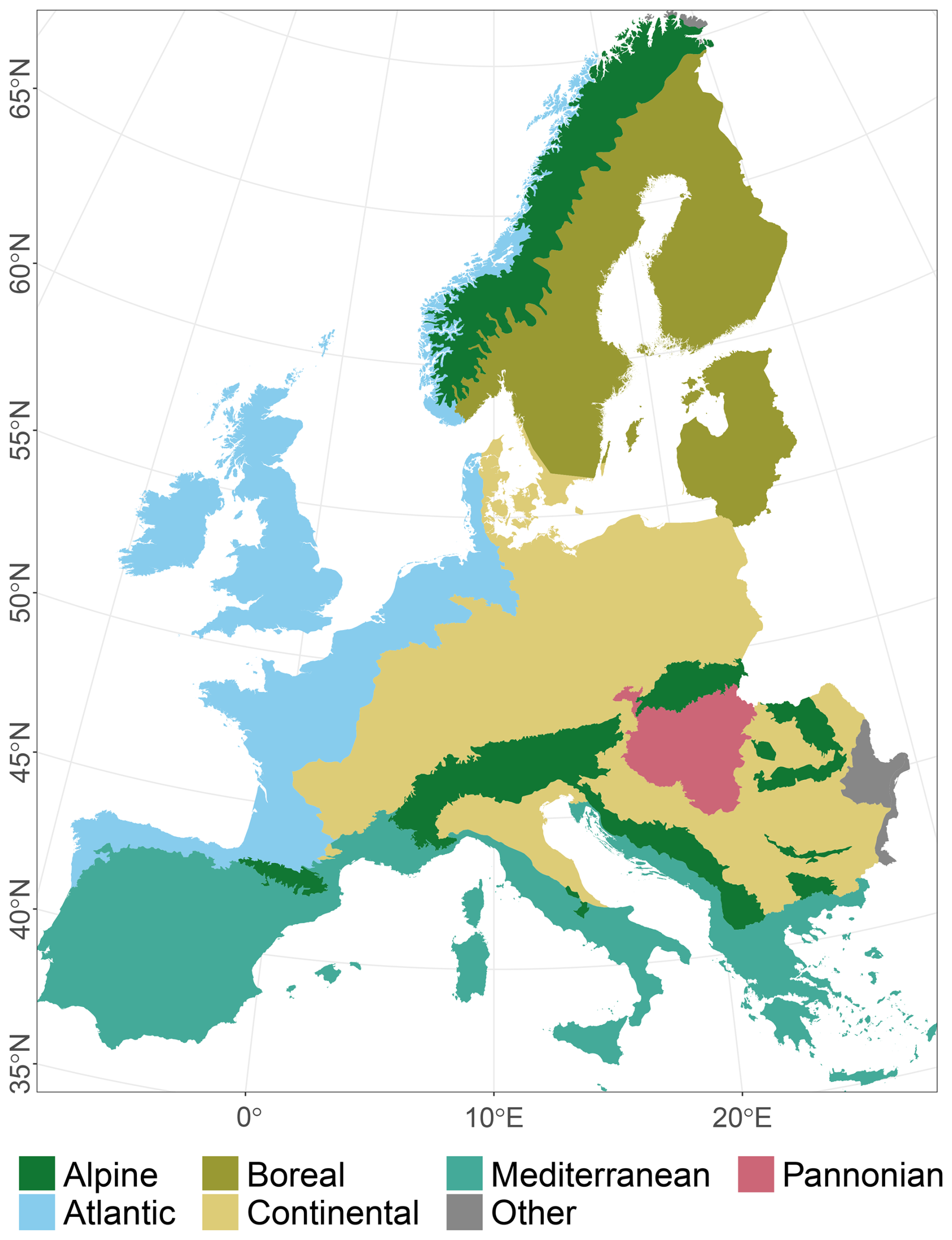
Figure 1 The study area with six biogeographical regions of Europe (EBRs), European Environment Agency (2016). The Arctic, Black Sea, and Steppic regions are combined into the group “Other” and will be omitted due to their small proportions.

2.1 Tree species data

We used the EU Joint Research Centre (JRC) tree species distributions as occurrence probabilities (De Rigo et al., 2016), ranging from 0 to 1, for our modelling procedure. They encompass 41 different tree species. All species show a zero-inflated beta distribution, usually with low occurrence probabilities in nonzero cases. These occurrence probability data are available in the ETRS89 Lambert azimuthal equal-area projection format, with a spatial resolution of 1 km. De Rigo et al. (2016) modelled these occurrence probabilities to derive spatially comprehensive distributions based on binary input data from various databases, such as national forest inventories. Due to their big-data modelling approach, outlier detection is negligible (see De Rigo et al., 2016, for further explanation). We chose to use these model outputs, as they offer spatially uniformly distributed occurrence probabilities. We are aware of potential model error propagation. However, this approach allows us to (a) apply various methods for cross-validation and reduction in spatial auto-correlation, as described in the following, and (b) model sparsely distributed tree species using these methods.

In total, we modelled all 41 available tree species (see Appendix Table C1). Invalid values within the dataset, such as −1, were eliminated. De Rigo et al. (2016) assigned any existing non-forest areas in the dataset a fill value of 0.0225 (Daniele De Rigo, personal correspondence, 2022), which we excluded from the subsequent modelling process. We chose to combine the occurrence probabilities of Quercus robur and Quercus petraea by retaining the maximum value per pixel, as both species are capable of hybridisation when co-occurring (Jensen et al., 2009; Gerber et al., 2014).

2.2 Bio-climatic data

The base data for the computation of the bio-climatic data are the EURO-CORDEX Coupled Model Intercomparison Project Phase 5 (CMIP5) climate simulations (Samaniego et al., 2022). These simulations include 88 realisations for the Intergovernmental Panel on Climate Change (IPCC) Representative Concentration Pathways (RCPs; IPCC, 2013) 2.6, 4.5, and 8.5, covering the years 1971 to 2098. Here, we used a slightly altered version of the reference and projection periods from Reichmuth et al. (2025).

Based on the existing literature, we selected 26 bio-climatic variables (Table 1). From all realisations belonging to one RCP, the 5th, 50th, and 95th percentiles of the bio-climatic variables were extracted for the projection periods (Fig. 2c1). For the reference period 1971 to 1990, we extracted the 50th percentiles of all 88 realisations. We grouped the combined realisations into five distinct time periods:

• 1971 to 1990 – reference

• 2021 to 2040 – projection

• 2041 to 2060 – projection

• 2061 to 2080 – projection

• 2079 to 2098 – projection due to data availability until 2098 and in order to maintain the period length of 20 years.

We downscaled the data from their original 3 km resolution to 1 km using the nearest-neighbour resampling method and reprojected them from WGS84 to the ETRS89 Lambert azimuthal equal area to match the resolution and projection of the other input data. We decided to limit the reference period to 1990 due to the substantial influence of climate change on the vegetation physiological responses, which was noticeable by the end of the 1980s (Chmielewski and Rötzer, 2001; Schaber and Badeck, 2005). As the tree species input data consider forests up to the year 2001 (De Rigo et al., 2016), we presumed that the stand was established in the 20th century and instead focused on historic climate conditions for our reference period. The remaining four time periods of 2021–2040, 2041–2060, 2061–2080, and 2079–2098 each mirror the reference period in length for the sake of consistency. The results presented in this paper are mainly focused on the 50th percentile for RCP 4.5. The results for RCP 2.6 and 8.5 can be accessed in Appendix D1. All computations here were done using the Python packages xclim (Bourgault, 2023a, b) and xarray (Hoyer et al., 2023).

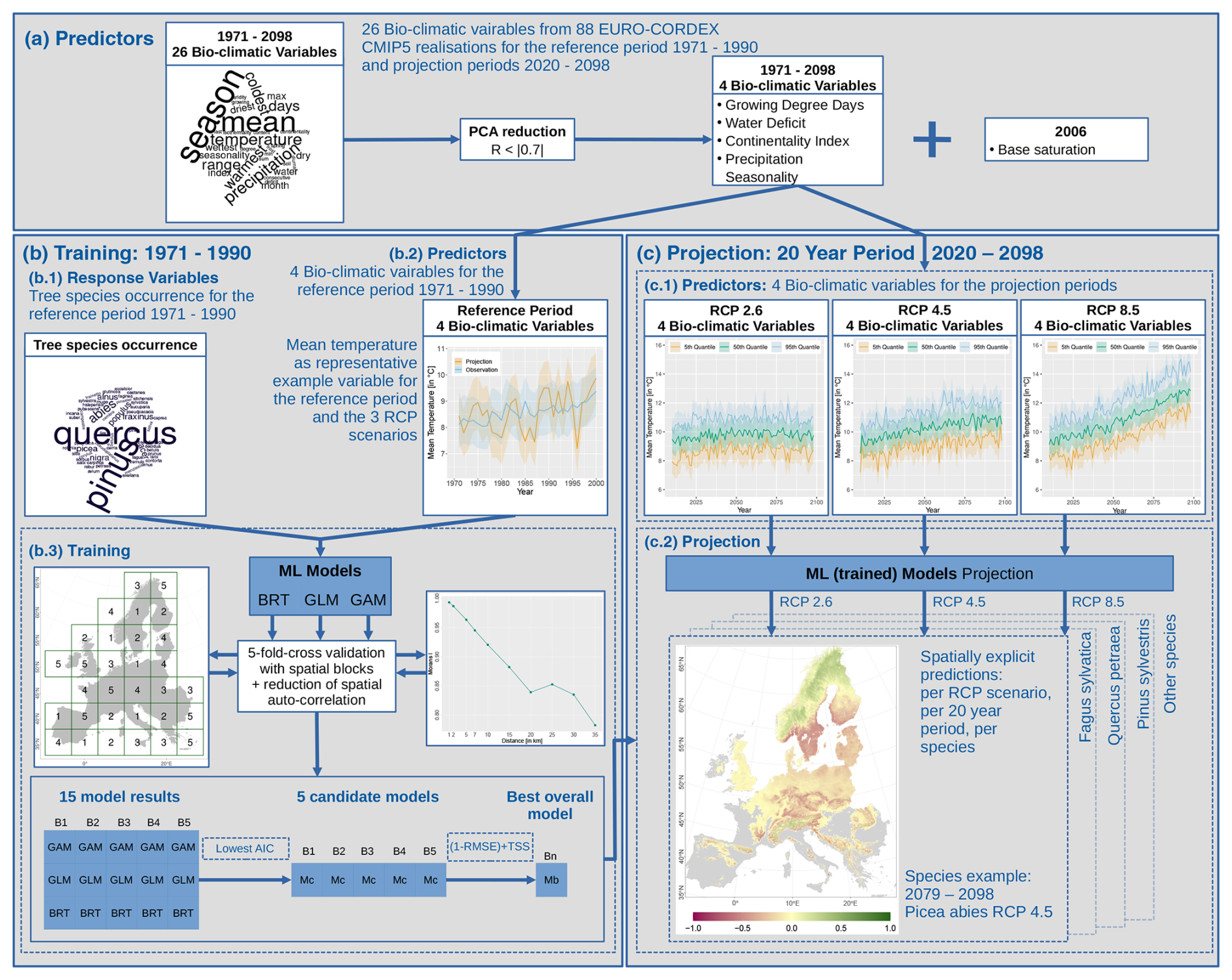
Figure 2 The modelling procedure outlined by a flowchart. In total, 26 bio-climatic variables serve as predictors for the reference period of 1971–1990 (a). To avoid over-parameterisation, they are reduced using a principal component analysis (PCA) and correlation analysis. The remaining bio-climatic variables (b1) are used as input in combination with tree species occurrence probabilities (b2) for training multiple statistical (machine learning, ML) models: boosted regression trees (BRTs), generalised linear models (GLMs), and generalised additive models (GAMs) (b3). Here, we applied spatial blocking for cross-validation and regular pixel spacing to reduce the spatial auto-correlation. Using the Akaike information criterion (AIC), we reduced the number of models to a set of candidate models (Mc) and finally one best overall model (Mb). The selected bio-climatic variables are extracted for the future climate scenarios RCP 2.6, 4.5, and 8.5 (c1), which we summarised in 20-year periods. These periods are used to project the tree species distribution using the best overall model (Mb) (c2).

2.3 Soil data

We used the chemical parameter base saturation from JRC “European Soil Database & soil properties” (Van Liedekerke et al., 2006; Panagos, 2006) as a predictor variable in the modelling procedure. This dataset is available in the ETRS89 Lambert azimuthal equal-area projection and at a 1 km spatial resolution.

2.4 Natura 2000 areas

We used N2K sites (European Environment Agency, 2021) in conjunction with the CORINE Land Cover map 2018 (European Environment Agency, 2019) to extract the forest cover within the protected areas. We used this information to select areas with a forest proportion ≥ 25 % and an extent ≥ 100 ha. These criteria were applied to 10 211 N2K sites. Per definition, more than one protected area – belonging to the Birds Directive or the Habitats Directive – can be reported for one and the same geographic location. This might lead to partial spatial overlap and may affect subsequent statistical derivations, which we were not able to correct for.

2.5 Variable selection

To reduce the chance of model overfitting, the bio-climatic variables were subjected to a principal component analysis (PCA; R (R Core Team, 2023) base function prcomp). We selected the first four principal components (PCs), as they cumulatively explained 90 % of the total variance. From each of these four PCs, the bio-climatic variables with the highest loading values (Fig. 3) in conjunction with botanical relevance were chosen as potential variables for the modelling procedure. A correlation analysis was then carried out using a correlation coefficient of $<\left|\mathrm{0.7}\right|$ as the threshold (Dormann et al., 2013) to avoid multicollinearity among the potential variables. From these potential variables, we selected growing degree days (PC1), water deficit (PC2) (Ohlemüller et al., 2006), continentality index (PC3) (Conrad, 1946), and precipitation seasonality (PC4) as predictor variables for the modelling procedure. We neglected bio-climatic variables of the type driest/wettest season, as they vary greatly within Europe and during the projection periods. We aggregated the selected bio-climatic variables to the mean and standard deviation per EBR for RCP 4.5 to show their trend over the time periods (Fig. B1 in Appendix B1). This trend shows a temperature increase and/or extension of the growing period of our simulation data over all EBRs (Fig. B1a). At the same time, differences between winter and summer temperatures decrease due to a lower continentality rate (Fig. B1b). Additionally, water deficit increases (Fig. B1c), which means that evapotranspiration exceeds precipitation. A similar trend can be observed for increasing precipitation seasonality, which allows the conclusion about distinct variation within the annual precipitation distribution (Fig. B1d).

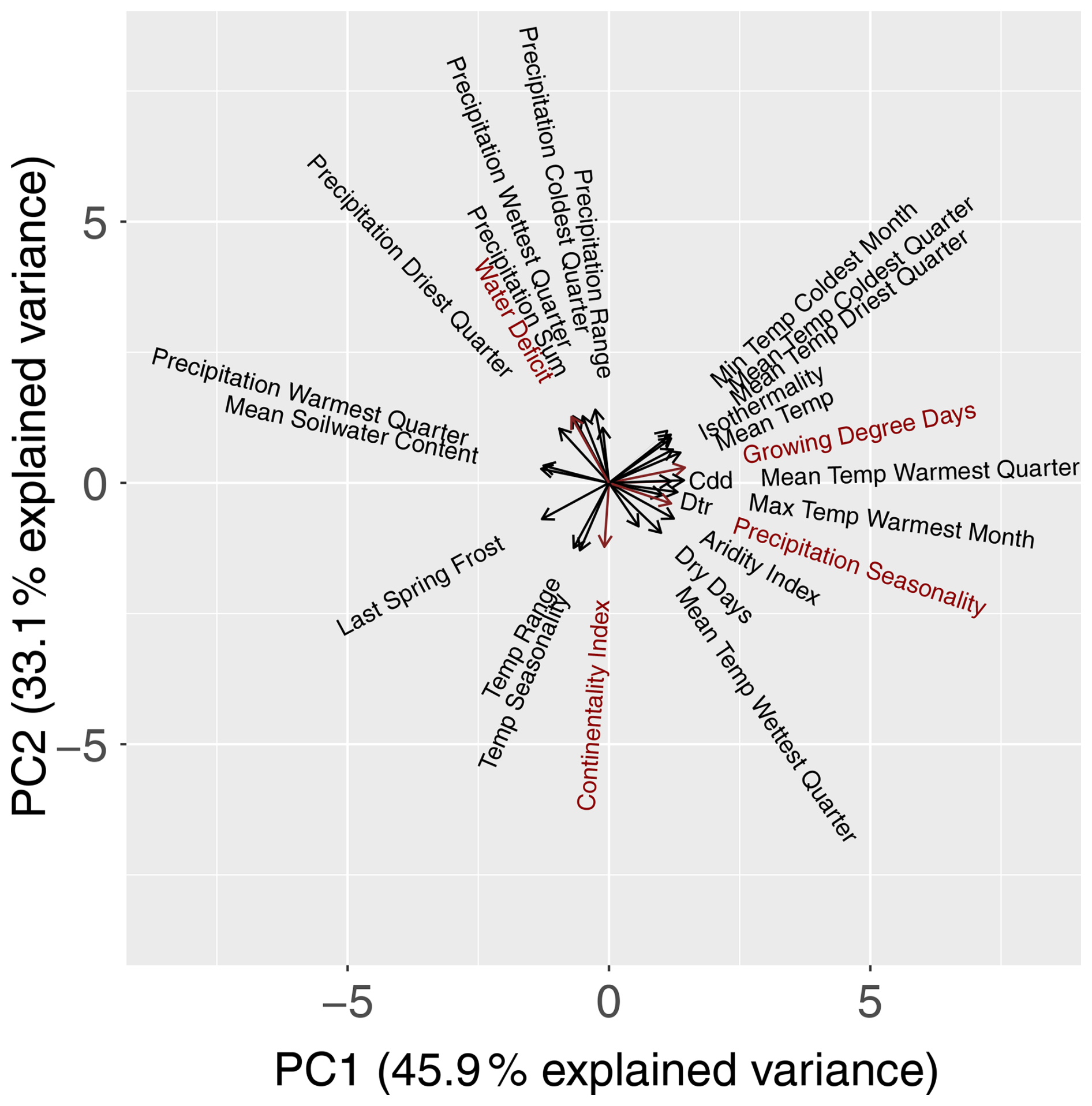
Figure 3 PCA biplot for all 26 bio-climatic variables. PC1 (x axis) and PC2 (y axis) explain 79 % of the variance. The length of the vectors (arrows) indicates the loading value. The longer the vector, the more information the variable carries. Close-by (opposite) vectors indicate a highly positive (highly negative) correlation. The selected bio-climatic variables are marked in red.

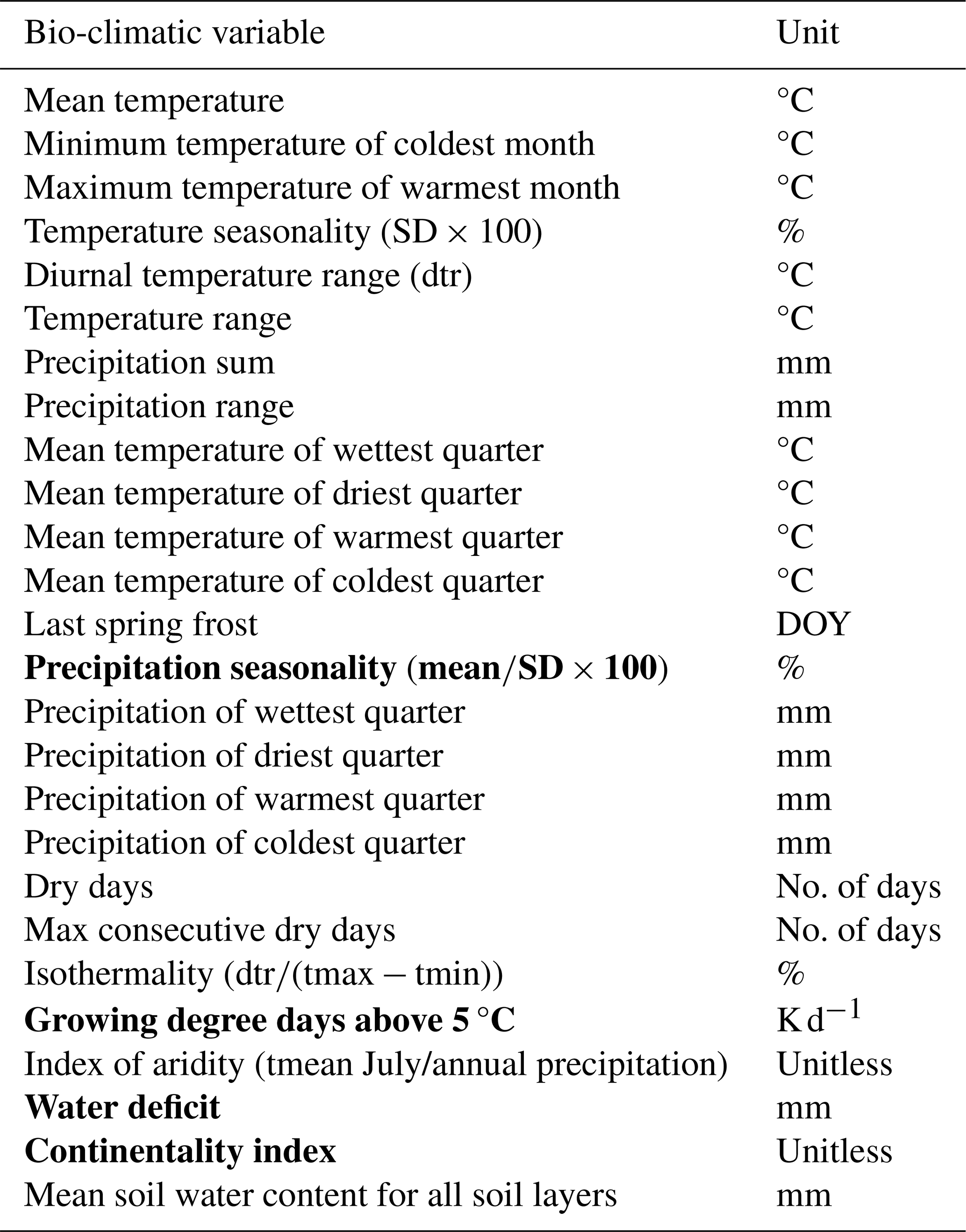
Table 1 The 26 bio-climatic variables, calculated for RCPs 2.6, 4.5, and 8.5. The variation in the 88 underlying realisations was accounted for using the 5th, 50th, and 95th percentiles. Bold rows indicate the selected bio-climatic variables used for the modelling procedure, as described in Sect. 2.5. Apart from common bio-climatic variables, we included water deficit (Ohlemüller et al., 2006) and continentality index (Conrad, 1946).

2.6 Cross-validation using spatial blocking

Spatial block separation is a useful procedure to divide modelling input data into evenly dispersed non-overlapping blocks for cross-validation (Roberts et al., 2017). Each data point is assigned to a block group that is used as either training or testing input for the model. This increases the transferability of the trained model to different regions. Using the R package blockcv (Valavi et al., 2019, 2023), we selected five randomly dispersed block groups with a 600×600 km extent per block and an equal data distribution among the groups (Fig. 4). We kept most default settings from the function cv_spatial and only changed the following: size = 600 000, iteration = 100, hexagon = FALSE, and offset = 0. During the modelling procedure, four out of five block groups were used for training, while the remaining block group was withheld for testing. This procedure was repeated five times so that all block groups served as testing data once (Fig. 2b3).

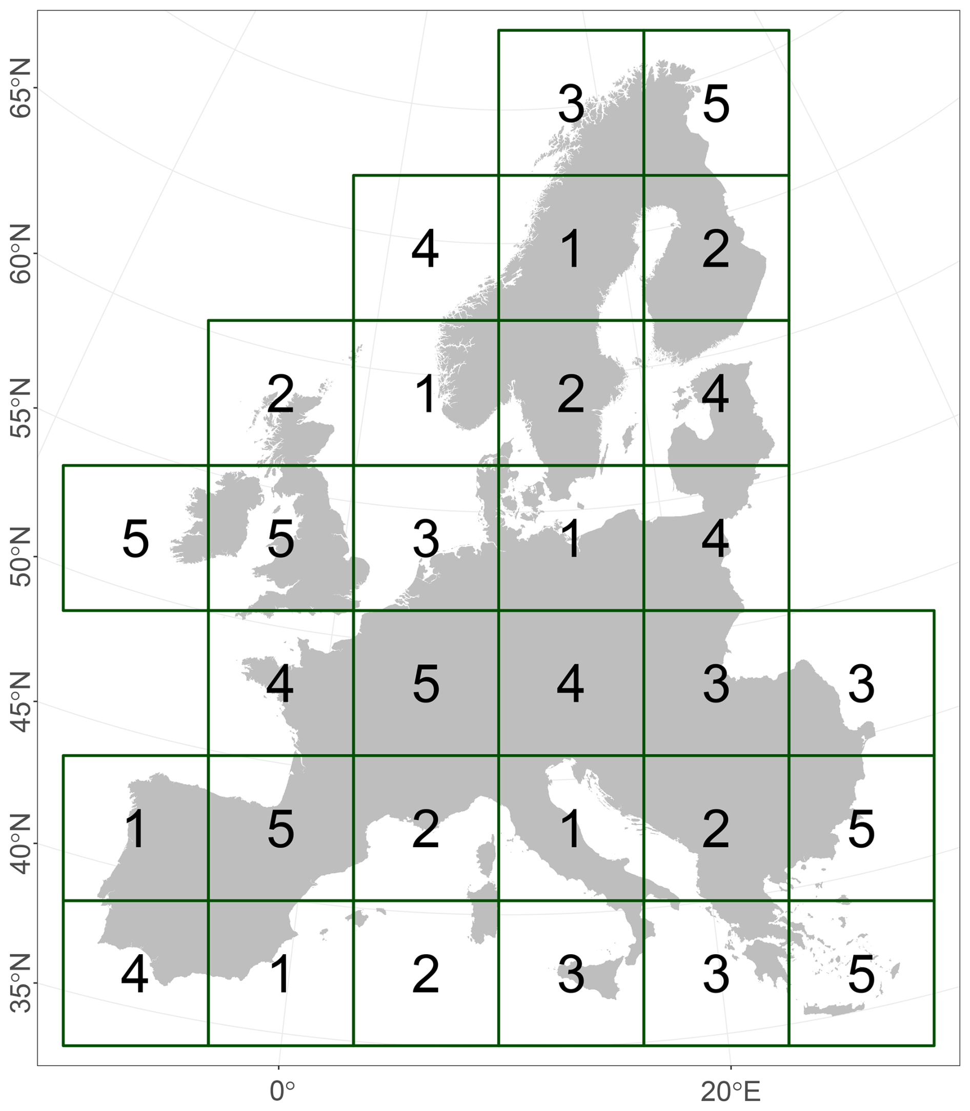
Figure 4 Spatial block distribution across Europe, with a block size of 600×600 km for cross-validation during the modelling procedure. Blocks with the same number belong to one group.

2.7 Reduction in spatial auto-correlation

Spatial auto-correlation can lead to (1) an overestimation of the predictive power of a trained model (Ploton et al., 2020), (2) inflated degrees of freedom with resulting false significant error probabilities, and (3) incorrect parameter estimates (Dormann, 2007). Among others, Dormann et al. (2007), Kühn (2007), and Ploton et al. (2020) corrected for the distribution of unequal residuals, which depend on the spatial auto-correlation, using computationally intensive methods. Even though we are aware of non-independent spatial observations, we have opted for a computationally cheap methodology, regular spatial distance separation. Hence, only data points that are spatially separated by a predefined distance were considered for the model training process. The distance assessment was based on global Moran's I estimations of model residuals using various distance values with the R package waywiser (Mahoney, 2023). The Moran's I range is $[-\mathrm{1},\mathrm{1}]$ and indicates strong auto-correlation in the form of clustered residuals (≫0), perfectly random data and thus no auto-correlation (∼0), or chequerboard-like dispersed data (<0). A regular distance of 20 km was selected as a trade-off between Moran's I estimates and a sufficient amount of training data (Fig. 5). The distance spacing was applied to the training data.

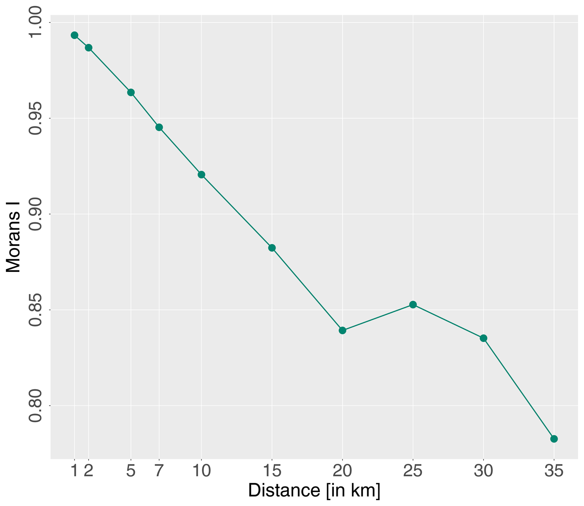
Figure 5 Moran's I of the Picea model residuals using GLMs and spatial distances of 1, 2, 5, 7, 10, 15, 20, 25, 30, and 35 km iterating over all five block groups and aggregated to their mean.

2.8 Statistical modelling

We modelled the potential distribution of each taxon using three well-established and widely used modelling algorithms: (1) generalised linear models (GLMs) (Nelder and Wedderburn, 1972), (2) generalised additive models (GAMs) (Hastie and Tibshirani, 1986), and (3) boosted regression trees (BRTs) (Friedman et al., 2000; Freund and Schapire, 1996; Friedman, 2001) (Fig. 2b). The corresponding R packages are stats (R Core Team, 2023) for GLMs, gam (Hastie, 2023) for GAMs, and dismo (Hijmans et al., 2022) (function gbm.step) for BRTs. First- and second-order polynomials of all predictor variables were included in the GLM and GAM. For the BRT, we used the default parameters but increased the number of initial trees (n.trees) from 50 to 100 for some performance gain, as the tree depth was rather high (5000 to 10 000), see Appendix Table A1 for parameter specifications. The tree species data serve as response variables; bio-climatic and soil data serve as predictor variables (Fig. 2b1 and b2). Only model runs in which the training data contained at least 200 nonzero data records were considered.

The model evaluation for each run was performed using the R package dismo (Hijmans et al., 2022). The evaluation parameters of interest were the Akaike information criterion (AIC) (Akaike, 1974), the true skill statistic (TSS) (Allouche et al., 2006), and the root-mean-square error for training vs. fitted values (RMSE). The TSS is an appropriate indicator of how well the model prediction fits the test data. The value range is $[-\mathrm{1},\mathrm{1}]$, where +1 indicates maximum agreement of model prediction vs. the test dataset, and values close to 0 indicate random performance of that model. Values <0 indicate that the opposite relationship would be better (i.e., coefficients multiplied by −1).

We trained 15 models in total: 5 block realisations × 3 algorithms (Fig. 2b3). We reduced these 15 models in two steps. (1) We took the best algorithm according to the lowest AIC score, which resulted in five candidate models, one for each block group. After the initial model runs and the candidate model selection, an evaluation of the model AIC (GLM, GAM) and feature importance (BRT) was used for model simplification. Here, the soil parameter base saturation was omitted from all models, as it had the lowest importance. In addition, we reduced the bio-climatic predictors where applicable. We calculated models with four and three bio-climatic variables and used the ones where delta AIC was >0. Similarly, the feature importance of the candidate BRT models using four bio-climatic predictors was evaluated. The least important predictor, with <10 %, was excluded if applicable. Hence, we only used the most appropriate and least parametric model. This model thinning for nonparametric BRT was applied for consistency with the GAM and GLM thinning approach. (2) From these candidate models, we selected the best-performing model M_b according to the sum of 1−RMSE_Mc and TSS_Mc (Eq. 1). They capture different aspects, but for transferability one needs both, recovering the observed pattern (large TSS) and at the same time minimising the error (low RMSE). Partial response curves of the final GAM model for Fagus with the three bio-climatic variables, continentality index, growing degree days, and water deficit, are shown in the Appendix Fig. C1. This best-performing model was used for projecting to the four projection periods (Fig. 2c). The projection outputs are pixel maps with a 1 km spatial resolution. The projection was applied to all three RCPs and all four projection periods (2021 to 2040, 2041 to 2060, 2061 to 2080, and 2079 to 2098) for the 5th, 50th, and 95th percentiles (see Sect. 2.2), as well as to the reference period of 1971 to 1990.

$$\begin{array}{}\text{(1)}& M_{\mathrm{b}}=max\left(\right(\mathrm{1}-{\mathrm{RMSE}}_{\mathrm{Mc}})+{\mathrm{TSS}}_{\mathrm{Mc}})\end{array}$$

2.9 Natura 2000 evaluation

To evaluate the potential effect of tree species distribution shifts at N2K sites, a change value (CV_i) was computed by taking occurrence probabilities per projection period (P_i(Time)) vs. projected reference (P_i(Reference)) per pixel i into account (Eq. 2). By relating this pixel-wise numerator to the overall maximum value within the projected reference (max(P(Reference))) as a denominator, we can extract the CV_i as the percentage of change. The change value range is $[-\mathrm{1},\mathrm{1}]$ and indicates an increase (P_i>0) or decrease (P_i<0) of the probabilities per projection period in comparison to the projected reference. Due to the intraspecific denominator, the CV_i can not be compared between the species but only within the projection periods per species. We extracted this change value for all pixels within each N2K site considered and aggregated them to a mean change value $\stackrel{\mathrm{‾}}{\mathrm{CV}}$ per N2K site (Eq. 3). We can use this information to quantify a potential tree species distribution change per N2K site. We then aggregated the median and 25th and 75th percentiles from all N2K site $\stackrel{\mathrm{‾}}{\mathrm{CV}}$ within an EBR. These metrics allow the quantification of the range of the shifts per EBR.

$$\begin{array}{}\text{(2)}& {\mathrm{CV}}_i={\displaystyle \frac{P_i\left(\mathrm{Time}\right)-P_i\left(\mathrm{Reference}\right)}{max\left(P\right(\mathrm{Reference}\left)\right)}},\end{array}$$

with CV_i as the change value per pixel, P_i(Time) as the probability of occurrence for the projection periods per pixel, P_i(Reference) as the probability of occurrence for the reference period per pixel, and max(P(Reference)) as the maximum probability of occurrence for the reference period.

$$\begin{array}{}\text{(3)}& \stackrel{\mathrm{‾}}{\mathrm{CV}}={\displaystyle \frac{\mathrm{1}}{n}}\sum _{i=\mathrm{1}}^n{\mathrm{CV}}_i\end{array}$$

3 Results

Here we present results of the statistical modelling (Sect. 3.1) and the N2K evaluation (Sect. 3.2) for the tree species Fagus, Picea, and Quercus.

3.1 Modelled species distributions

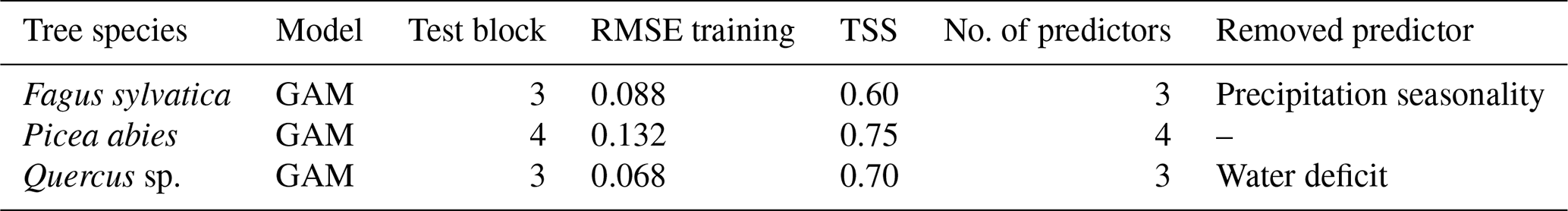
GAM was the overall best-performing model (Table 2) for the taxa Fagus, Picea, and Quercus (Appendix Table C1 for all 41 tree species). The predictor reduction from four to three predictors was applicable for Fagus and Quercus. The TSS values vary from 0.60 (Fagus) to 0.75 (Picea) to 0.70 (Quercus). The shifts in occurrence probability vary depending on the species and region.

Table 2 The best model evaluation result for species Fagus, Picea, and Quercus. The test block column indicates the block that was omitted during the training process. The RMSE training column is the RMSE calculated based on training data vs. model fit, whereas TSS is calculated based on testing data and values predicted by the model. The no. of predictors and removed predictor columns show whether a predictor was removed during the training procedure and if so, which one.

The projected reference period reveals very similar distribution patterns to those of the actual input data (Figs. 6a, 7a, and 8a vs. 6b, 7b, and 8b). The occurrence probabilities, however, are lower. The projection period of 2079 to 2098 for RCP 4.5 shows small changes compared to the reference period for Fagus (Fig. 6c). On the other hand, Picea and Quercus reveal a severe decline throughout the study area (Figs. 7c and 8c). Fagus declines in lowland areas across Europe (Fig. 6d), while it increases in the foothills of mountain ranges. In order to quantify these changes, we have to consider the change value range of $[-\mathrm{1},\mathrm{1}]$, which cancels itself out during mean change value calculation. We have therefore calculated the absolute mean change value and also the mean above 0 as well as the mean below 0 to reveal gain and loss. This results in a 6 % absolute mean change value (−6 % mean loss, 8 % mean gain). Similarly, Quercus shows a severe decline in western Europe, as well as in the Pannonian and Mediterranean areas, and further shifts into the Scandinavian countries, Finland, the Baltic countries, and higher elevations (Fig. 8d). This accounts for a 23 % absolute mean change value (−28 % mean loss, 21 % mean gain). For Picea, we can see a severe decline in most areas in central Europe, Baltic countries, and southern Norway/Sweden/Finland (Fig. 7d). The taxon increases in northern Norway/Sweden/Finland and in the central Alps. In general, lowland areas are affected by losses, whereas the taxon shifts into higher elevations and northern areas. This accounts for a 17 % absolute mean change value (−17 % mean loss, 18 % mean gain). The results for RCP 2.6 and RCP 8.5 are included in the Appendix and show either less pronounced (RCP 2.6 Figs. C2, C3, and C4) or more pronounced development (RCP 8.5 Figs. C5, C6, and C7).

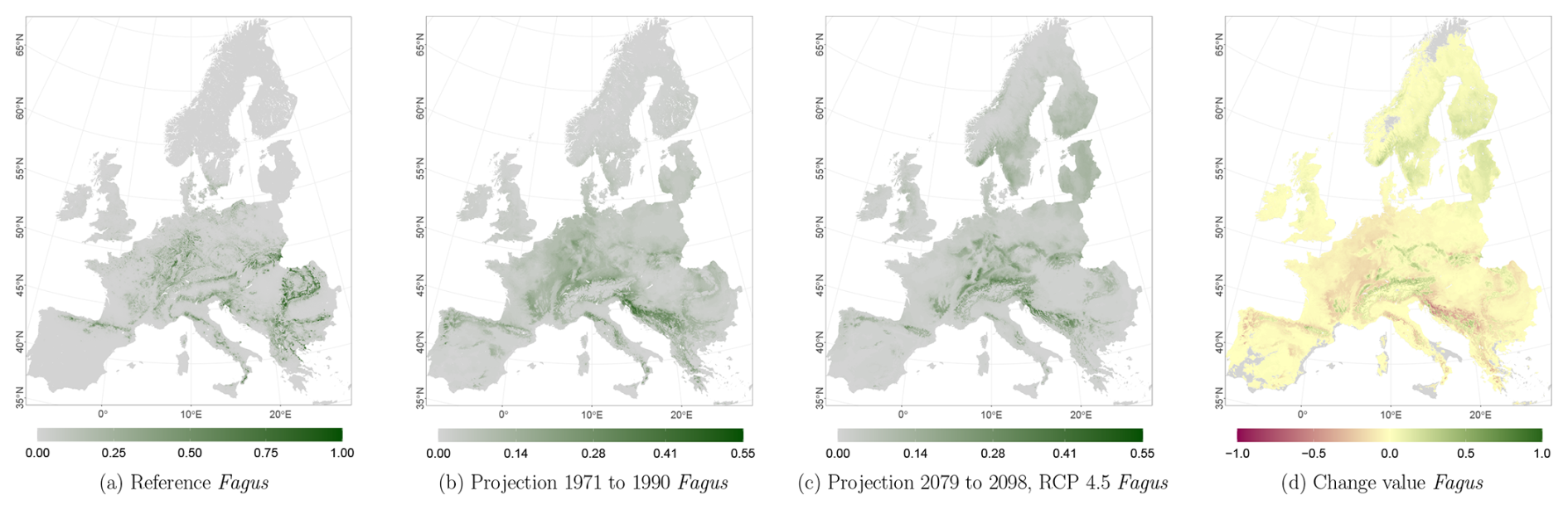
Figure 6 Occurrence probability for Fagus sylvatica. Panel (a) shows the reference data (JRC tree species occurrences (De Rigo et al., 2016)), panel (b) is the model projection for the reference period of 1971 to 1990, and panel (c) shows model projections for the 2079 to 2098 RCP 4.5 at the 50th percentile. Panel (d) indicates the change value, a proportional difference for the projection 2079 to 2098 vs. the projected reference. Here magenta reveals loss, green shows gain, yellow reveals no change in abundance, and grey indicates that the species is not present in reference or in projection data.

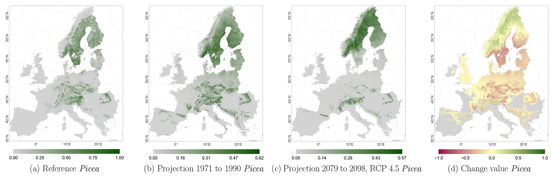
Figure 7 Occurrence probability for Picea abies. Panel (a) shows the reference data (JRC tree species occurrences (De Rigo et al., 2016)), panel (b) is the model projections for the reference period of 1971 to 1990, and panel (c) shows model projections for the 2079 to 2098 RCP 4.5 at the 50th percentile. Panel (d) indicates the change value, a proportional difference for the projection 2079 to 2098 vs. the projected reference. Here magenta reveals loss, green shows gain, yellow reveals no change in abundance, and grey indicates that the species is not present in reference or in projection data.

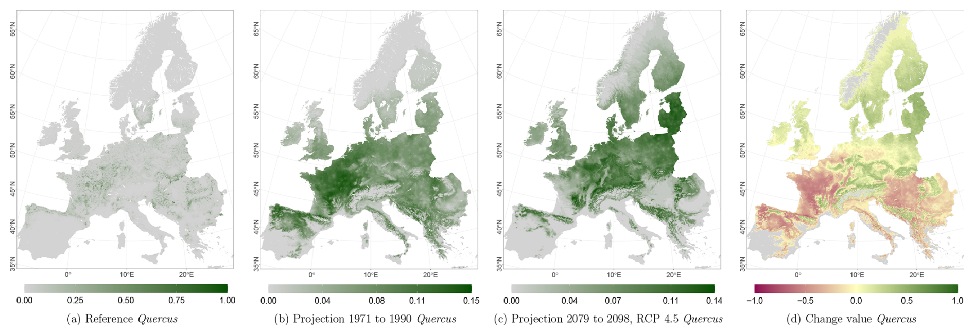
Figure 8 Occurrence probability for Quercus sp. Panel (a) shows the reference data (JRC tree species occurrences (De Rigo et al., 2016)), panel (b) is the model projections for the reference period 1971 to 1990, and panel (c) shows model projections for the 2079 to 2098 RCP 4.5 at the 50th percentile. Panel (d) indicates the change value, a proportional difference for the projection 2079 to 2098 vs. the projected reference. Here magenta reveals loss, green shows gain, yellow reveals no change in abundance, and grey indicates that the species is not present in reference or in projection data.

3.2 Effects on Natura 2000 sites

At the N2K sites across Europe, Fagus shows again the least decline in the three modelled taxa and showed increases in lower and higher mountain ranges such as the Ore mountains and the Alps, Tatras, and Carpathians (Fig. 9a). Aggregating the change over the study area, it accounts for 8 % of the absolute mean change value (−7 % mean loss, 9 % mean gain) until 2098 for RCP 4.5. On the other hand, Picea potentially loses ground at the N2K sites in these mountainous regions (Fig. 9c). In contrast, that taxon reveals a strong increase in Scandinavia and Finland as it moves further north and into higher elevations. Aggregated over all N2K sites, Picea reveals a mean absolute change value of 18 % (−18 % mean loss, 15 % mean gain) until 2098, taking RCP 4.5 into account. Quercus shows a decline at N2K sites of the Mediterranean, France, and the Pannonian area, as well as increases in central Europe, lower mountain ranges, Finland, and the Baltic countries (Fig. 9e). The overall mean absolute change value until 2098 amounts to 23 % (−23 % mean loss, 24 % mean gain).

Focusing on the EBRs, we can see similar trends. Fagus reveals an increase at N2K sites in the Alpine and Boreal regions, while it decreases in the Atlantic, Continental, Mediterranean, and Pannonian regions (Fig. 9b). Only a few outliers show a negative or positive change value of $<-\mathrm{50}$ % or >50 % (Alpine and Continental EBRs). However, Picea shows a negative trend in all EBRs (Fig. 9d). The trend in the Boreal and Alpine regions is quite severe, as some whiskers (1.5×interquartile range) exceed −50 % towards the end of the century. Quercus, however, again shows a similar pattern to Fagus, with positive trends in the Alpine and Boreal regions and negative trends in the remaining EBRs (Fig. 9f). However, here also some whiskers exceed 50 % or −50 %.
RCPs 2.6, 4.5, and 8.5 reveal similar trends per species and EBR (Tables D1, D2, and D3 in Appendix D1) over all periods. The negative as well as positive trends continue over time and RCPs. They partly exceed change values of 50 % or −50 %, e.g., Quercus at the 75th and 25th percentile for RCP 8.5. The plot results for RCPs 2.6 and 8.5 can be accessed in Appendix Figs. D1 and D2.

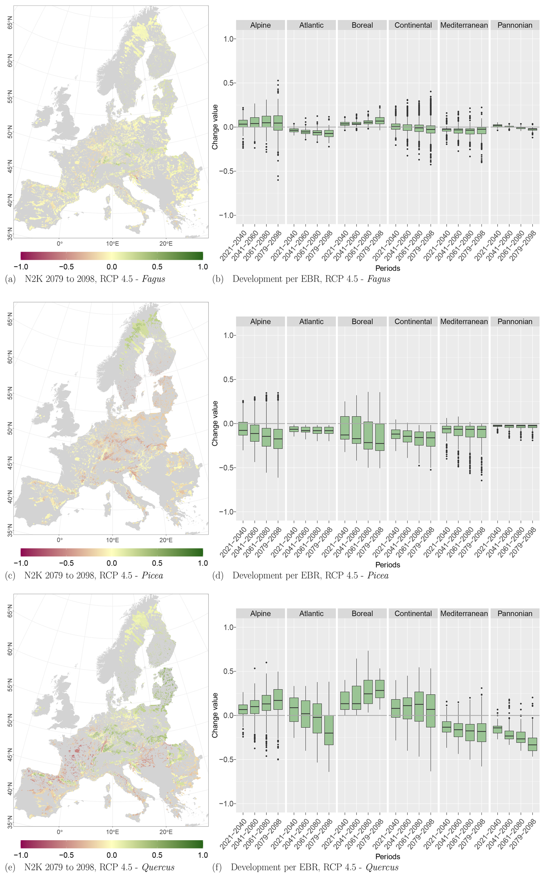
Figure 9 Change values for Picea, Fagus, and Quercus, aggregated to the mean per N2K site with forest cover ≥25 % and size ≥100 ha. Panels (a), (c), and (e) show the period for the 2079 to 2098 RCP 4.5 at the 50th percentile. Negative change values presented in dark magenta reveal a decline, which means that the species was present in the reference period but is no longer present in the projection period. The green colour or positive change values indicate increasing abundance in this area. Yellow (change values of 0) indicates no change in abundance, and grey indicates that the species is present in neither the reference period nor the projection period. Panels (b), (d), and (f) show the change value development over all periods and the RCP 4.5 projection for the EBRs.

4 Discussion

Our results reveal substantial shifts in tree species' probabilities of occurrence towards the end of the century under warming climate conditions according to the IPCC RCP 4.5 scenario. The combination of decreasing precipitation during the vegetation period with increasing temperatures and/or longer vegetation periods can lead to diminished species-specific site adaptation.

4.1 Shifts in tree species distribution

Based on past studies, we would expect the main distributional shifts to be in the lowlands, but we would also expect species-dependent shifts within elevated areas and at higher latitudes. Our results can confirm the overall species distribution trend from other modelling studies (Buras and Menzel, 2019; Hinze et al., 2023; Hickler et al., 2012; Thuiller et al., 2005) but differ in some aspects, especially for Quercus and Fagus. Fagus experiences the lowest distribution changes, which is contradictory to findings by Mathys et al. (2021), who found the strongest climatically induced effect (mortality) for Fagus. In our study, Quercus instead gains abundance distinctively in the Boreal and Alpine EBRs, with simultaneous losses in the Atlantic, Mediterranean, and Pannonian EBRs. Similar results were found by Thuiller (2004) and confirmed by Hickler et al. (2012), who revealed the greatest changes in arctic and alpine regions. The trend in bio-climatic variables can lead to reduced growth, especially for Picea, as this cold-adapted taxon reveals a strong dependency on summer precipitation and responds more negatively to higher summer temperatures in comparison to thermophilic Quercus species (Zang et al., 2012) or Fagus (Obladen et al., 2021; Pretzsch et al., 2020). This is confirmed by Thuiller et al. (2005): warm-adapted species have higher chances for an increase in their range extent than cold-climate-adapted species. Also, the maps reveal an increasing occurrence probability for Quercus in warmer regions, while Picea migrate to higher elevations and latitudes, which is in line with Araújo et al. (2011). Fagus shows higher drought and heat sensitivity compared to other co-existing tree species and reveals a reduction in competitive strength under unfavourable conditions (Leuschner, 2020; Scharnweber et al., 2011). Among the three species analysed, Quercus showed the most gain, but on the other hand, this taxon also revealed the most severe losses. However, Brandl et al. (2020) revealed similar survival/mortality rates for Quercus and Fagus.

Modelled species distributions from Mauri et al. (2022) reveal very similar trends for the three taxa. They used binary input data regarding tree species occurrence but similar climate data as well as model algorithms (BRT, GAM, and GLM, among others), which means that their study can serve as an appropriate verification study. Consequently, differences between our study and the abovementioned ones (Mathys et al., 2021, Hickler et al., 2012, and Hinze et al., 2023) might stem from several factors such as the input data and/or model algorithms employed, as well as methods for optimising the modelling procedure, such as a reduction in spatial auto-correlation and block cross-validation. These factors concern the spatiotemporal resolution and spatial extent employed. The implementation of interspecific interactions and species behaviour scenarios such as dispersal can also influence the model outcome significantly, which we did not implement here. Beyond the climate conditions used in SDM, other parameters such as potential land use change can influence the species distribution potential and diminish the quantitative comparability of studies.

4.2 Effect of tree species shift at forested Natura 2000 sites and their conservation goals

Considering these species shifts, we can quantify the potential changes in species distributions for forested N2K sites (≥25 % forest cover and ≥100 ha extent). In our study, we assess the change value for N2K sites to quantify potential gains and losses in the occurrence probabilities, taking current forest tree species distributions into account. In particular, consideration of the current tree species distributions is essential, as the definition of N2K sites relies on current species-specific habitats. Our approach allows us to pinpoint areas where tree species occurrences might change without considering the entire habitat since habitats will not remain intact when single species migrate in and out. Severe changes in Quercus and Picea can influence the prevalence of character species and the associated conservation goal.

Parmesan and Yohe (2003) found a possible expansion of temperate species with a simultaneous decline in polar species distributions. Ackerly et al. (2010) even infer that climates with retracting extent could lead to a decrease in species abundance and an increasing extinction risk of species adapted to such climatic conditions, which is questioned by Sporbert et al. (2020). Nevertheless, climate-induced species shifts can lead to severe economic losses as well as ecological ones, and the early (anticipatory) planting of possible non-European replacement tree species is recommended (Hanewinkel et al., 2012). As non-European species conflict with the Habitats Directive, suitable tree species should be considered in order to maintain the conservation objectives. Recently, potential replacement species in forest management (Mauri et al., 2023) and also the climate potential of tree species throughout the century (Wessely et al., 2024) were analysed without a focus on conservation areas.

The response to potential habitat losses generally involves more conservation efforts or alterations in habitat definition rather than the removal of the conservation status. The ultimate goal of the Habitats Directive is to prevent species extinction and to protect endangered habitats. This often requires ongoing and increasing efforts (Hermoso et al., 2019) and adjustments to conservation strategies. A political debate on how to deal with climate-change-induced alterations at forest N2K sites is ongoing. De Koning et al. (2014) derived three main points of discourse: (1) further enforcement by more strict policies, (2) taking dynamic effects within the N2K sites into account, and (3) maintaining the current policy until new scientific evidence allows changes. Cabeza and Moilanen (2001), Hannah et al. (2002), Hermoso et al. (2019), Mawdsley et al. (2009), and Root et al. (2003) endorse the second point of discourse by considering biodiversity dynamics and potential species shift when designing conservation areas. Biodiversity is undergoing natural transformations due to shifts in species distribution (Pressey et al., 2007), and historically defined habitat status cannot prevail through climate change (Baatar et al., 2019). Araújo et al. (2011) even conclude that N2K sites do not preserve climate suitability for species or do so less effectively than in unprotected areas due to less management; they demand new and adapted strategies. Hermoso et al. (2019) recommend amending N2K sites' conservation goals and defining protected species in a dynamic way based on their International Union for Conservation of Nature (IUCN) Red List threat status. An alteration of species composition or structure in a habitat is not necessarily to be regarded as deterioration (European Commission and Directorate-General for Environment, 2013). Therefore, European Commission and Directorate-General for Environment (2013) recommend an adaptive management strategy for the site management plans to face the direct and indirect effects of climate change. Araújo et al. (2011) also mention integrated management for the area surrounding the N2K sites to allow species movement between protected areas. Nevertheless, the conservation efforts in the EU lack financial, personal, and political support (Hermoso et al., 2019).

We support this demand and recommend a dynamic definition of habitat conservation goals similar to those of Hermoso et al. (2019) within existing or new N2K sites, as our results reveal significant species shifts and thus potentially severe habitat changes for Picea and Quercus. These species cannot remain in areas with unfavourable climatic conditions, especially in the Boreal, Alpine, Mediterranean, and Atlantic EBRs. This development will affect Annex II habitat types where these taxa are defined as typical species and thus will also affect dependent Annex I species with the protected status. We do not recommend a spatially dynamic definition of N2K sites itself as socioeconomic conflicts (Hermoso et al., 2019) (e.g., with other land use types) interfere with conservation goals and species distribution.

4.3 Methodological constraints and limitations

Most species distribution studies that we refer to use binary (i.e., presence/absence or presence-only) input data. Our species input data are spatially uniformly distributed occurrence probabilities with a value range of [0,1] and reveal a zero-inflated beta distribution that leads to reduced projection probabilities that never reach 1, [0,1). The change value, which we calculated, is species-specific and reflects the change in relation to the projected reference data. This allows a trend comparison but no alignment to absolute values across studies. The variable reduction is intended to reduce model complexity based on statistical inference, such as AIC evaluation. Neglecting the soil variable base saturation was necessary, as it revealed lowest variable importance within the models. This is contrary to Walthert and Meier (2017) and Pompe et al. (2008), who found improved statistics by including edaphic parameters. It is possible that the relatively coarse information content within the base saturation layer (three classes) has led to the insignificant importance within the models. In general, species distribution models attempt to map important elements of the n-dimensional hyperspace of Hutchinson's niche (Hutchinson, 1957) by deriving a statistical relationship between the occurrence of a species and the environmental variables. Distribution modelling presumes species climate equilibrium to be their input state (Guisan et al., 1999; Pearson and Dawson, 2003). But this does not include the influence of forest management with reduced competition and delayed species reaction to changes in climatic conditions. The prevalence of a certain tree species in the current climate does not necessarily imply that these conditions are the most favourable for that species. In particular, pure stands with heavy forest management can also occur in areas with less suitable site conditions, such as the economically important Picea. This could affect the niche that is realised and thus the modelling results (Pearson and Dawson, 2003).

4.4 Conclusion

Our study highlights the significant influence of tree species distribution shifts on forested N2K sites across Europe. Major tree species distribution changes have potential negative effects on the N2K integrity, an EU-wide conservation area network. Although the European Commission enables and encourages an adaptive management of N2K sites, the static protection regime counteracts the dynamic nature of climate impacts. We therefore advocate for a more dynamic definition of the conservation objectives that takes climate-driven changes in tree species distributions into account, particularly in relation to Annex I and Annex II protected species and habitats. Cold-adapted Picea in particular reveals a severe decline at forested N2K sites throughout Europe, which emphasises the need for dynamic conservation goals. Future research should explore and evaluate potential surrogate tree species that satisfy the conservation goals in a changing climate and provide important ecosystem services for the society. These findings should provide valuable guidance for decision-makers to ensure the effectiveness of the conservation efforts.

Appendix A

A1 ODMAP standard protocol

(Reichmuth, 2024)(Helmholtz-Centre for Environmental Research, 2024)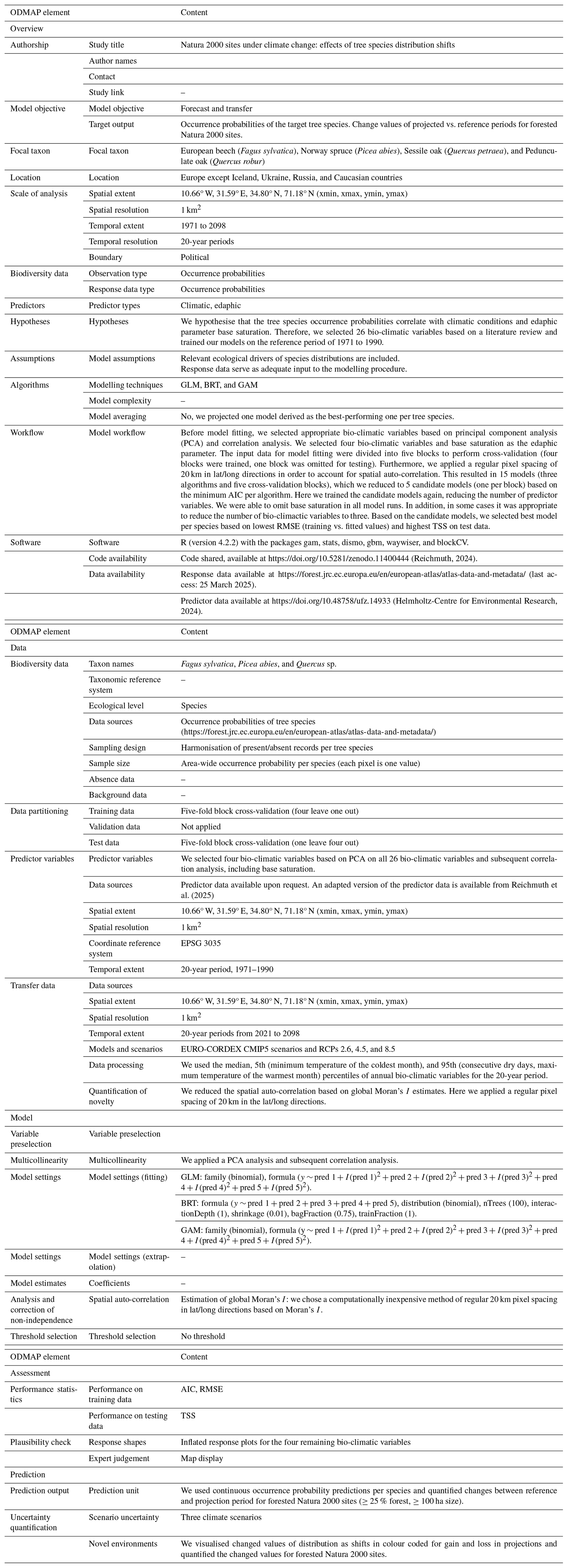

Table A1 ODMAP 1.0 standard protocol (Zurell et al., 2020), including mandatory fields.

Appendix B

B1 Bio-climatic variables

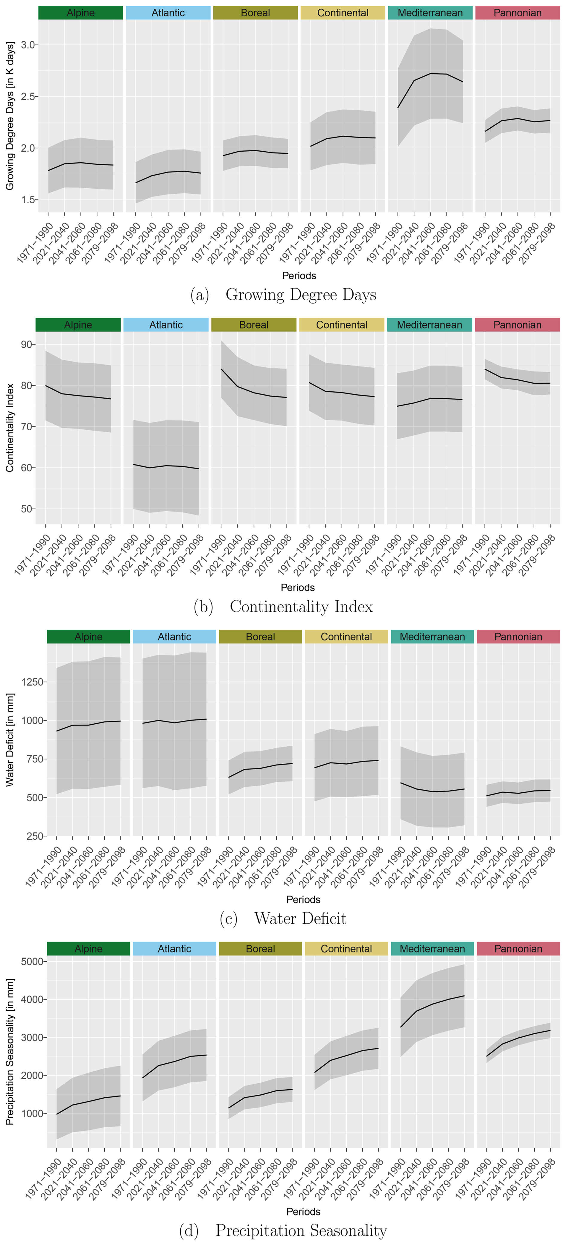
Figure B1 Trend for selected bio-climatic variables over the reference and projection periods (RCP 4.5, 50th percentile) for the EBRs. Black lines indicate the mean values, and the grey areas show the corresponding standard deviations.

Appendix C

Table C1 Model evaluation results for the best model and for all 41 tree species.

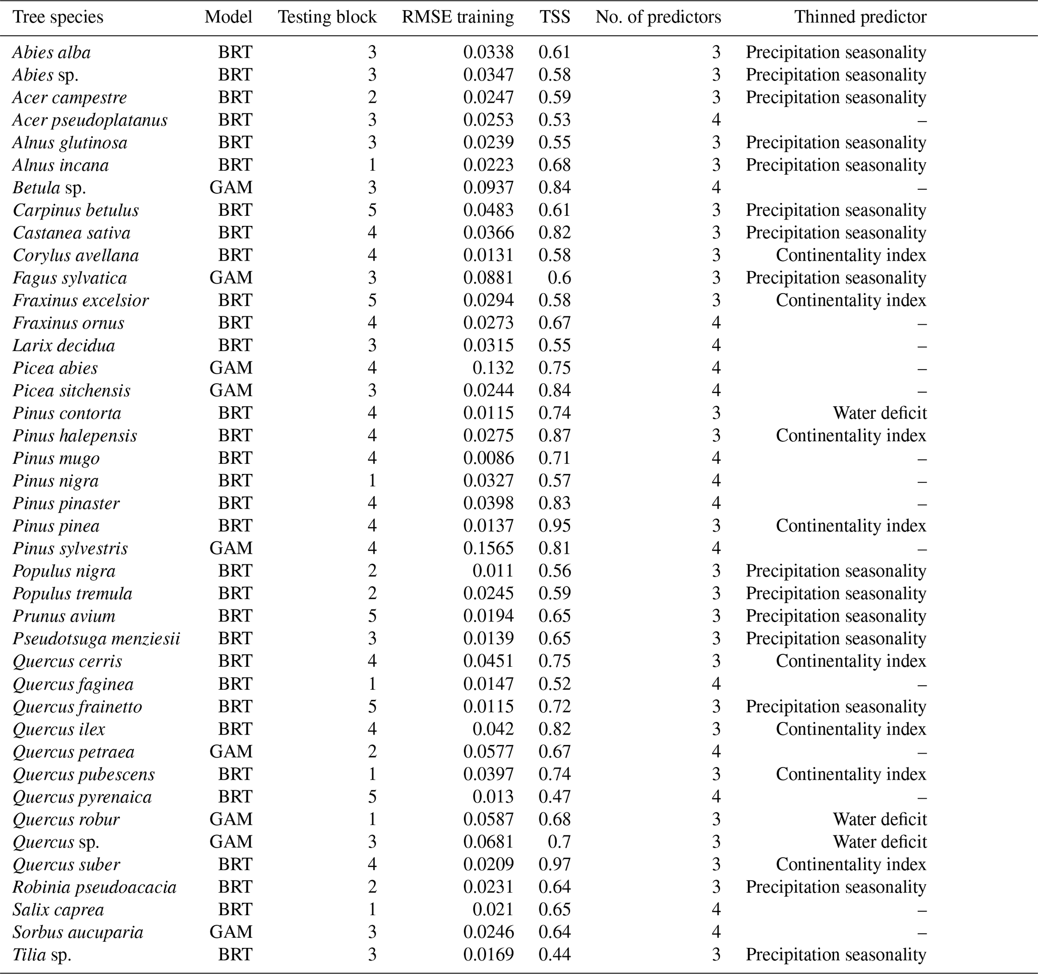
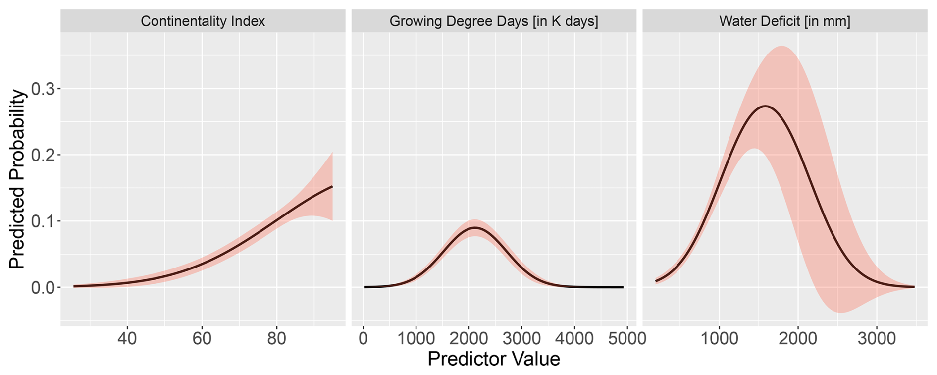
Figure C1 Partial response curves of the final GAM model for Fagus with the three bio-climatic variables: continentality index, growing degree days, and water deficit. The response curves show the fitted taxon–variable relationship along the entire gradient.

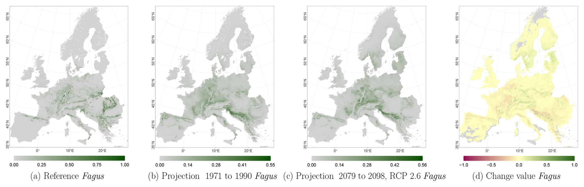
Figure C2 Occurrence probability for Fagus. Panel (a) shows the reference data (JRC tree species occurrences (De Rigo et al., 2016)), panel (b) is the model projection for the reference period of 1971 to 1990, and panel (c) shows model projections for the 2079 to 2098 RCP 2.6 at the 50th percentile. Panel (d) indicates the change value, a proportional difference for the projection 2079 to 2098 vs. the projected reference. Here magenta reveals loss, green shows gain, yellow reveals no change in abundance, and grey indicates that the species is not present in reference or in projection data.

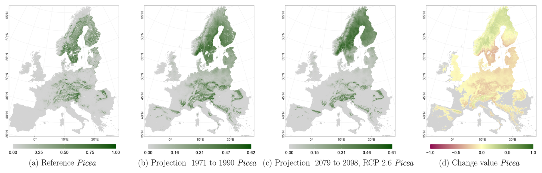
Figure C3 Occurrence probability for Picea. Panel (a) shows the reference data (JRC tree species occurrences (De Rigo et al., 2016)), panel (b) is the model projection for the reference period of 1971 to 1990, and panel (c) shows model projections for the 2079 to 2098 RCP 2.6 at the 50th percentile. Panel (d) indicates the change value, a proportional difference for the projection 2079 to 2098 vs. the projected reference. Here magenta reveals loss, green shows gain, yellow reveals no change in abundance, and grey indicates that the species is not present in reference or in projection data.

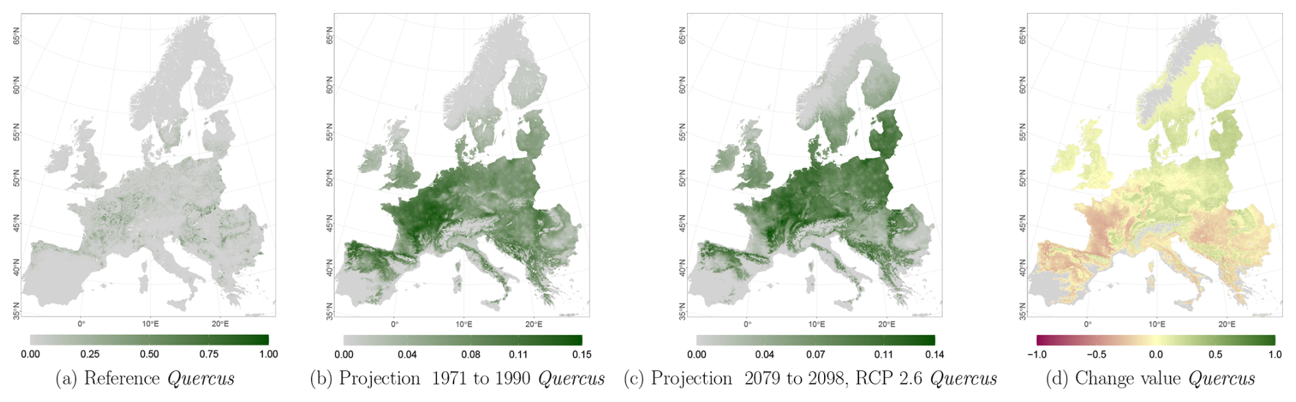
Figure C4 Occurrence probability for Quercus. Panel (a) shows the reference data (JRC tree species occurrences (De Rigo et al., 2016)), panel (b) is the model projection for the reference period of 1971 to 1990, and panel (c) shows model projections for the 2079 to 2098 RCP 2.6 at the 50th percentile. Panel (d) indicates the change value, a proportional difference for the projection 2079 to 2098 vs. the projected reference. Here magenta reveals loss, green shows gain, yellow reveals no change in abundance, and grey indicates that the species is not present in reference or in projection data.

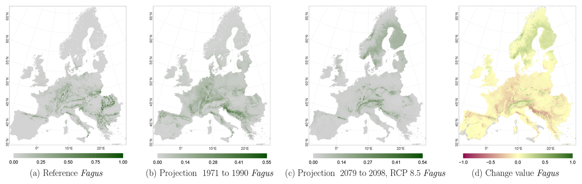
Figure C5 Occurrence probability for Fagus. Panel (a) shows the reference data (JRC tree species occurrences (De Rigo et al., 2016)), panel (b) is the model projection for the reference period of 1971 to 1990, and panel (c) shows model projections for the 2079 to 2098 RCP 8.5 at the 50th percentile. Panel (d) indicates the change value, a proportional difference for the projection 2079 to 2098 vs. the projected reference. Here magenta reveals loss, green shows gain, yellow reveals no change in abundance, and grey indicates that the species is not present in reference or in projection data.

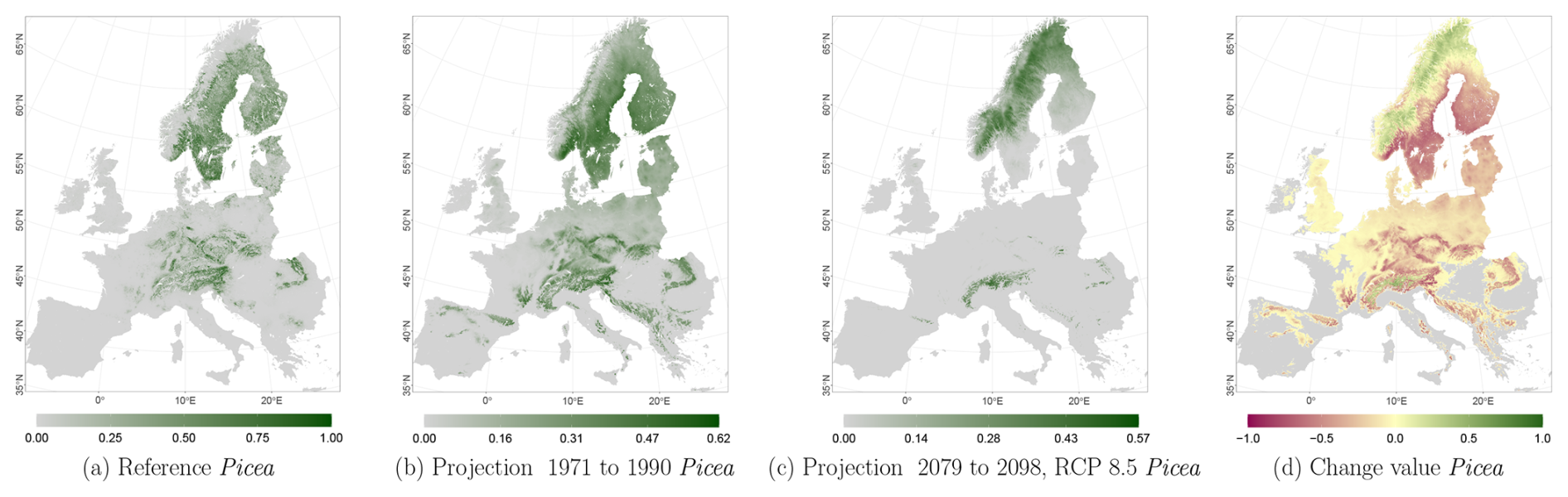
Figure C6 Occurrence probability for Picea. Panel (a) shows the reference data (JRC tree species occurrences (De Rigo et al., 2016)), panel (b) is the model projection for the reference period of 1971 to 1990, and panel (c) shows model projections for the 2079 to 2098 RCP 8.5 at the 50th percentile. Panel (d) indicates the change value, a proportional difference for the projection 2079 to 2098 vs. the projected reference. Here magenta reveals loss, green shows gain, yellow reveals no change in abundance, and grey indicates that the species is not present in reference or in projection data.

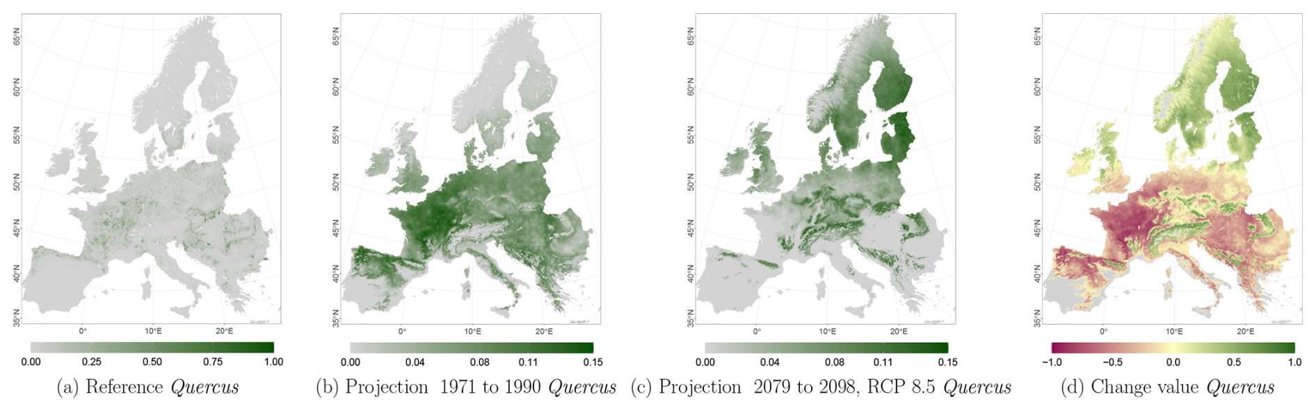
Figure C7 Occurrence probability for Quercus. Panel (a) shows the reference data (JRC tree species occurrences (De Rigo et al., 2016)), panel (b) is the model projection for the reference period of 1971 to 1990, and panel (c) shows model projections for the 2079 to 2098 RCP 8.5 at the 50th percentile. Panel (d) indicates the change value, a proportional difference for the projection 2079 to 2098 vs. the projected reference. Here magenta reveals loss, green shows gain, yellow reveals no change in abundance, and grey indicates that the species is not present in reference or in projection data.

Appendix D

D1 N2K quantification

Table D1 Natura 2000 change value statistics (in $\mathit{\%}\cdot {\mathrm{10}}^{-\mathrm{2}}$) per EBR, period, and RCP for Fagus sylvatica for the 50th percentile. The median and 25th and 75th percentile metrics are provided to show the variance.

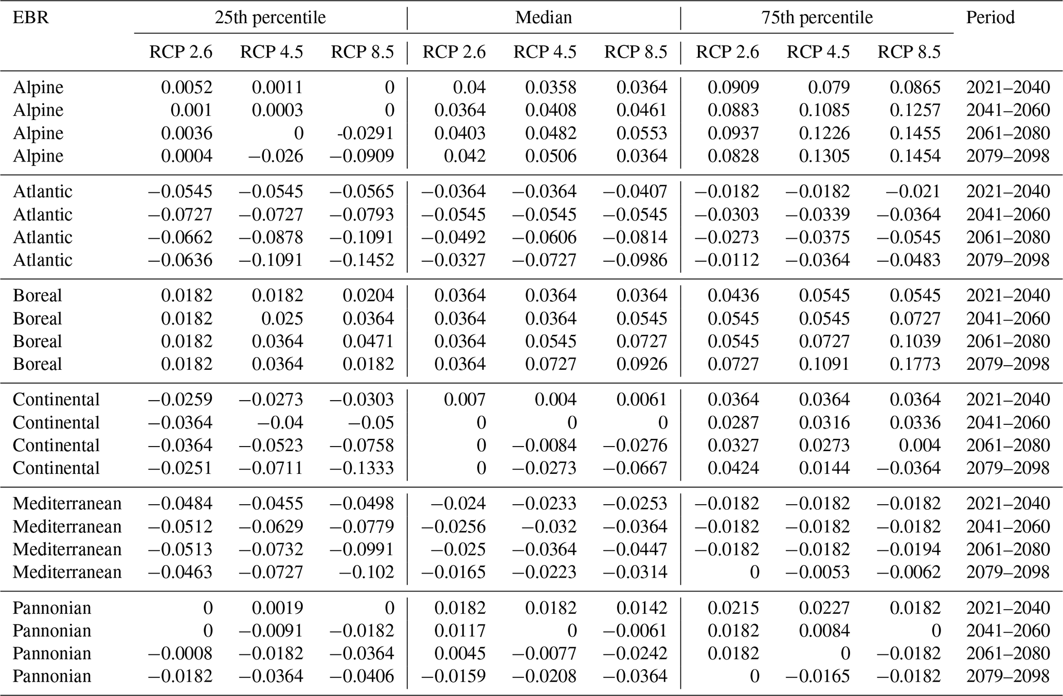
Table D2 Natura 2000 change value statistics (in $\mathit{\%}\cdot {\mathrm{10}}^{-\mathrm{2}}$) per EBR, period, and RCP for Picea abies for the 50th percentile. The median and 25th and 75th percentile metrics are provided to show the variance.

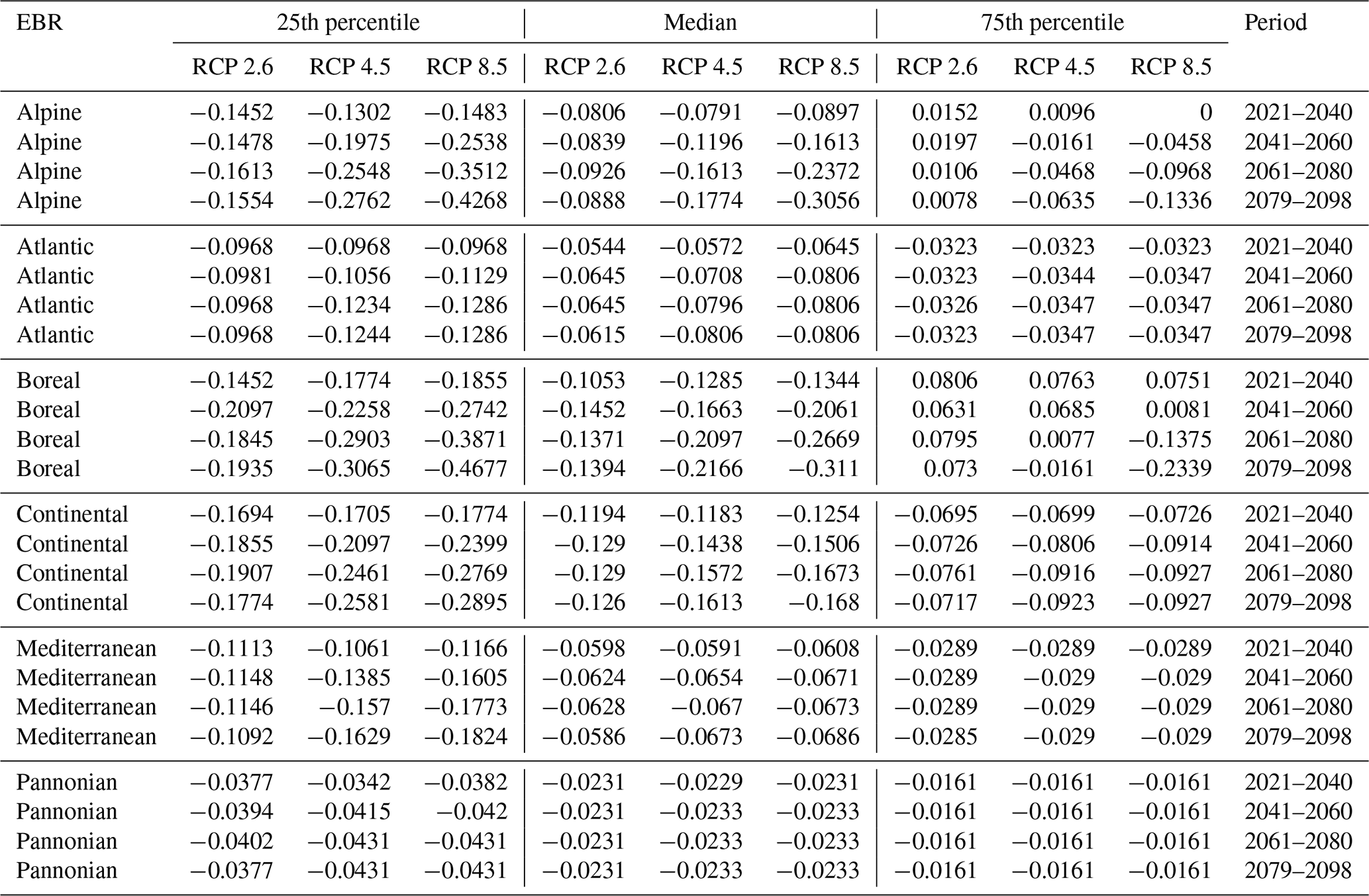
Table D3 Natura 2000 change value statistics (in $\mathit{\%}\cdot {\mathrm{10}}^{-\mathrm{2}}$) per EBR, period and RCP for Quercus sp. for the 50th percentile. The median and 25th and 75th percentile metrics are provided to show the variance.

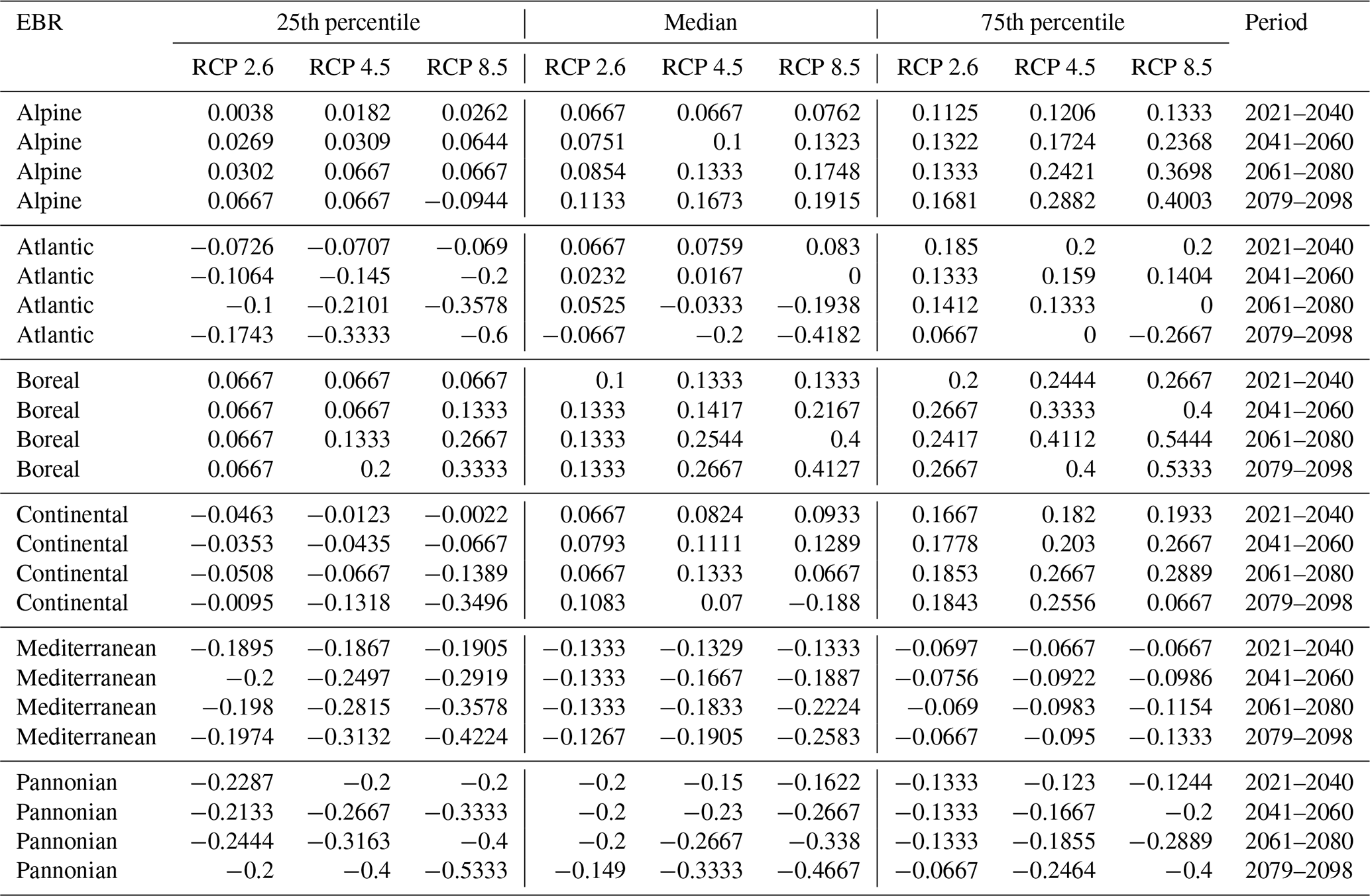
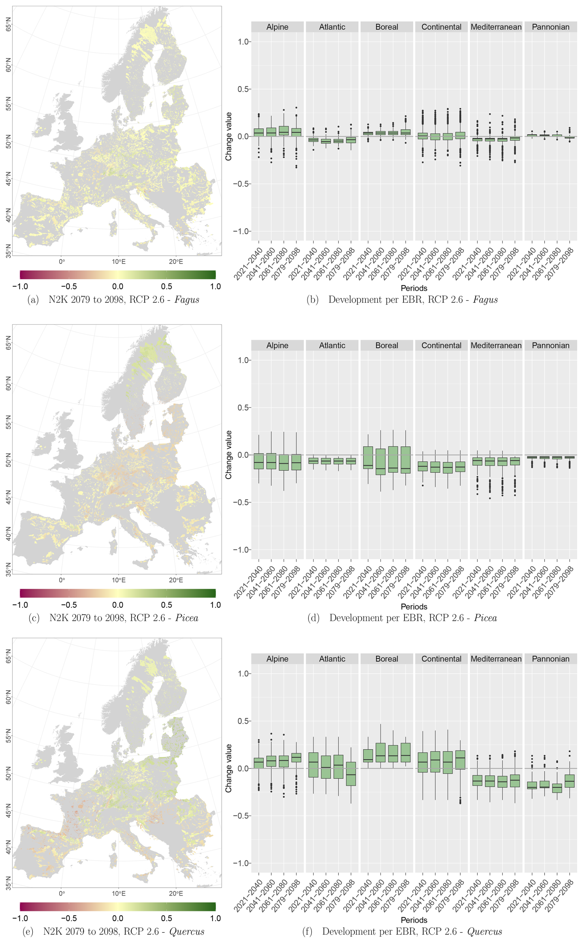
Figure D1 Change values for Picea, Fagus, and Quercus, aggregated to the mean per N2K site with forest cover ≥25 % and size ≥100 ha. Panels (a), (c), and (e) show the period for the 2079–2098 RCP 2.6 at the 50th percentile. Negative change values presented in dark magenta reveal a decline, which means that the species was present in the reference period but is no longer present in the projection period. The green colour or positive change values indicate increasing abundance in this area. Yellow (change values of 0) indicates no change in abundance, and grey indicates that the species is present in neither the reference period nor the projection period. Panels (b), (d), and (f) show the change value development over all periods and the RCP 2.6 projection for the EBRs.

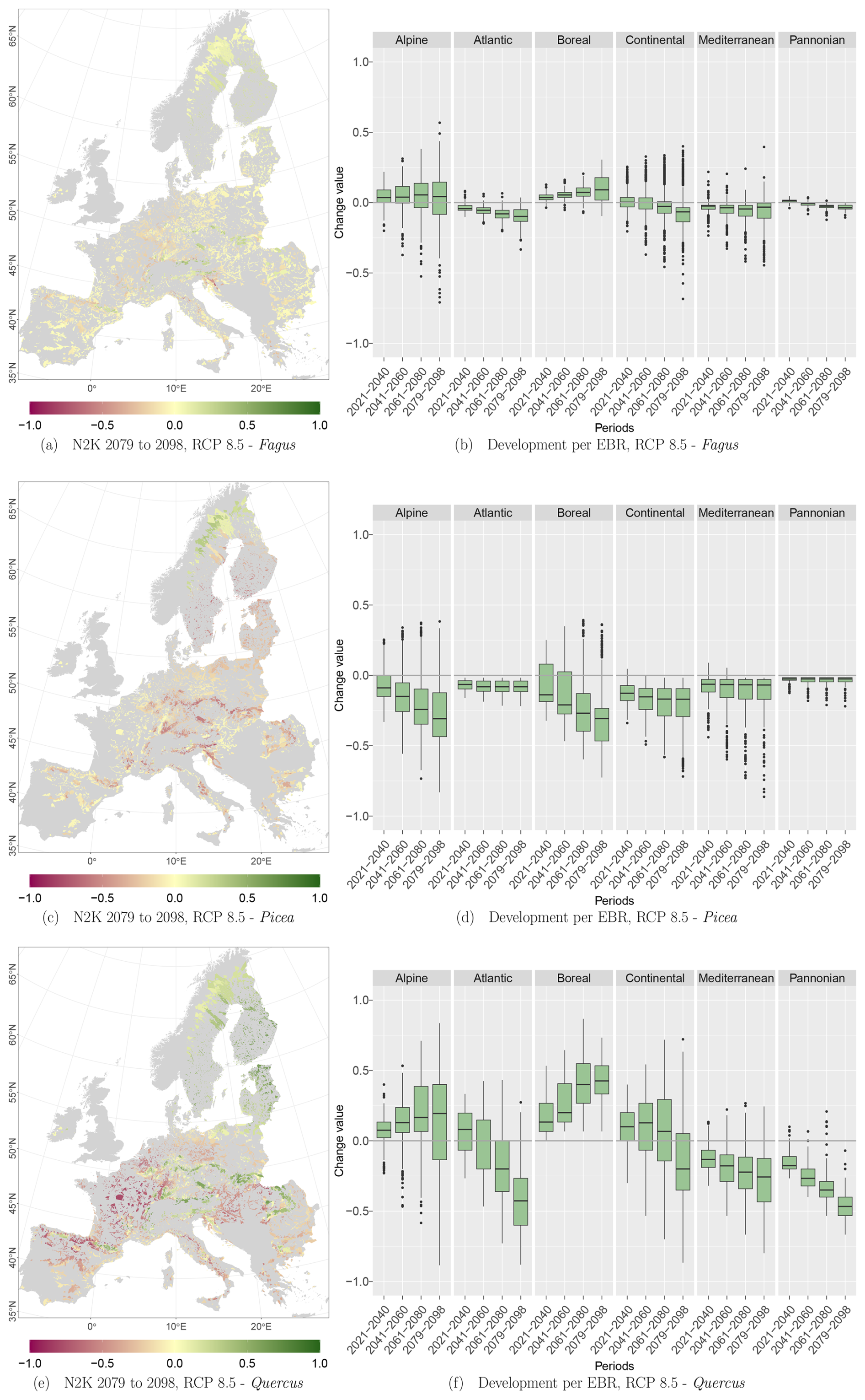
Figure D2 Change values for Picea, Fagus, and Quercus, aggregated to the mean per N2K site with forest cover ≥25 % and size ≥100 ha. Panels (a), (c), and (e) show the period for the 2079–2098 RCP 8.5 at the 50th percentile. Negative change values presented in dark magenta reveal a decline, which means that the species was present in the reference period but is no longer present in the projection period. The green colour or positive change values indicate increasing abundance in this area. Yellow (change values of 0) indicates no change in abundance, and grey indicates that the species is present in neither the reference period nor the projection period. Panels (b), (d), and (f) show the change value development over all periods and the RCP 8.5 projection for the EBRs.